Python image processing: frequency domain filtering, noise reduction and image enhancement

Image processing has become an integral part of our daily lives, involving various fields such as social media and medical imaging. Images obtained from digital cameras or other sources such as satellite photos and medical scans may require preprocessing to remove or enhance noise. Frequency domain filtering is a possible solution that can remove noise while enhancing image sharpening.

Fast Fourier Transform (FFT) is a mathematical technique that transforms images from the spatial domain to the frequency domain. It is a key tool for frequency transformation in image processing. By leveraging a frequency domain representation of an image, we can effectively analyze the image based on its frequency content, thereby simplifying the application of filtering procedures to remove noise. This article will discuss the various stages involved in the frequency transformation of an image from FFT to inverse FFT, combined with the use of FFT shift and inverse FFT shift.

This article uses three Python libraries, namely openCV, Numpy and Matplotlib.

import cv2
 import numpy as np
 from matplotlib import pyplot as plt
 img = cv2.imread('sample.png',0) # Using 0 to read image in grayscale mode
 plt.imshow(img, cmap='gray')#cmap is used to specify imshow that the image is in greyscale
 plt.xticks([]), plt.yticks([])# remove tick marks
 plt.show()

1. Fast Fourier Transform (FFT)

Fast Fourier Transform ( FFT) is a widely used mathematical technique that allows images to be converted from the spatial domain to the frequency domain and is a basic component of frequency transformation. Using FFT analysis, the periodicity of the image can be obtained and divided into different frequency components to generate an image spectrum that displays the amplitude and phase of each image's respective frequency component.

f = np.fft.fft2(img)#the image 'img' is passed to np.fft.fft2() to compute its 2D Discrete Fourier transform f
 mag = 20*np.log(np.abs(f))
 plt.imshow(mag, cmap = 'gray') #cmap='gray' parameter to indicate that the image should be displayed in grayscale.
 plt.title('Magnitude Spectrum')
 plt.xticks([]), plt.yticks([])
 plt.show()

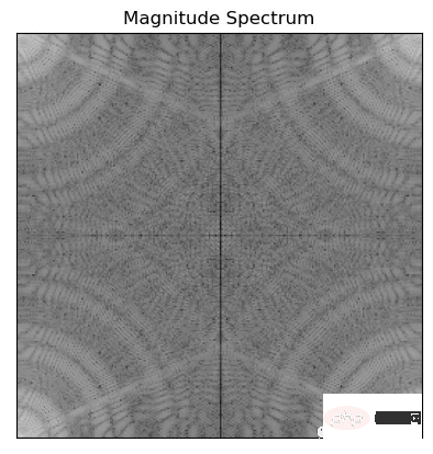
The above code uses np.abs() to calculate the amplitude of Fourier transform f, np.log() Convert to a logarithmic scale and multiply by 20 to get the amplitude in decibels. This is done to make the amplitude spectrum easier to visualize and interpret.

2. FFT shift

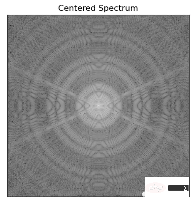
In order to apply the filtering algorithm to the image, FFT shift is used to move the zero frequency component of the image to the center of the spectrum

fshift = np.fft.fftshift(f)
 mag = 20*np.log(np.abs(fshift))
 plt.imshow(mag, cmap = 'gray')
 plt.title('Centered Spectrum'), plt.xticks([]), plt.yticks([])
 plt.show()

3. Filtering

One of the purposes of frequency transformation is to use various filtering algorithms to reduce noise and improve image quality. The two most commonly used image sharpening filters are the Ideal high-pass filter and the Gaussian high-pass filter. These filters all use the frequency domain representation of the image obtained through the Fast Fourier Transform (FFT) method.

Ideal high-pass filter (ideal filter) is an infinitely long filter with infinite frequency bandwidth and ideal passband and stopband responses. Signals of all frequencies within its passband are completely transmitted, while signals of all frequencies within its stopband are completely suppressed.

In the frequency domain, the amplitude-frequency response of an ideal filter is:

• In the passband, the amplitude-frequency response is 1
• In the stopband, The amplitude-frequency response is 0

In the time domain, the impulse response of the ideal filter is:

• In the passband, the impulse response is an infinite Unit impulse function sequence
• In the stop band, the impulse response is zero

Since the ideal filter has infinite bandwidth in the frequency domain, it cannot be implemented in practical applications . The digital filters used in practice are usually based on the approximation of the ideal filter, so they are just an Ideal.

The Gaussian high-pass filter is a filter commonly used in digital image processing. Its function is to retain high-frequency detail information in the image and suppress low-frequency signals. This filter is based on a Gaussian function and has a smooth frequency response that can adapt to a variety of image details.

The frequency response of the Gaussian high-pass filter can be expressed as:

H(u,v) = 1 - L(u,v)

Where, L(u, v) is a low-pass filter, which can be represented by a Gaussian function. The response of a high-pass filter is obtained by subtracting the response of the low-pass filter from 1. In practice, different parameter settings are usually used to adjust the Gaussian function to achieve different filtering effects.

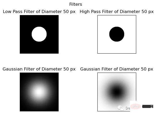
Circular masks (disk-shaped images) are used to define the frequency components to be retained or suppressed when Fourier transform is performed in the image. In this context, an ideal filter usually refers to an ideal low-pass or high-pass filter that can be selected in the frequency domain to retain or suppress signals within a specific frequency range. After applying this ideal filter to the Fourier transform of the image, and then performing the inverse transformation, the image processed by the filter can be obtained.

We won’t introduce the specific details, let’s look at the code directly:

The following function is to generate a circular mask for ideal high-pass and low-pass filters

import math
 def distance(point1,point2):
 return math.sqrt((point1[0]-point2[0])**2 + (point1[1]-point2[1])**2)
 
 def idealFilterLP(D0,imgShape):
 base = np.zeros(imgShape[:2])
 rows, cols = imgShape[:2]
 center = (rows/2,cols/2)
 for x in range(cols):
 for y in range(rows):
 if distance((y,x),center) < D0:
 base[y,x] = 1
 return base
 
 def idealFilterHP(D0,imgShape):
 base = np.ones(imgShape[:2])
 rows, cols = imgShape[:2]
 center = (rows/2,cols/2)
 for x in range(cols):
 for y in range(rows):
 if distance((y,x),center) < D0:
 base[y,x] = 0
 return base

The following function generates a Gaussian high and low pass filter with the required circular mask

import math
 def distance(point1,point2):
 return math.sqrt((point1[0]-point2[0])**2 + (point1[1]-point2[1])**2)
 
 def gaussianLP(D0,imgShape):
 base = np.zeros(imgShape[:2])
 rows, cols = imgShape[:2]
 center = (rows/2,cols/2)
 for x in range(cols):
 for y in range(rows):
 base[y,x] = math.exp(((-distance((y,x),center)**2)/(2*(D0**2))))
 return base
 
 def gaussianHP(D0,imgShape):
 base = np.zeros(imgShape[:2])
 rows, cols = imgShape[:2]
 center = (rows/2,cols/2)
 for x in range(cols):
 for y in range(rows):
 base[y,x] = 1 - math.exp(((-distance((y,x),center)**2)/(2*(D0**2))))
 return base

Filtering example

fig, ax = plt.subplots(2, 2) # create a 2x2 grid of subplots
 fig.suptitle('Filters') # set the title for the entire figure
 
 # plot the first image in the top-left subplot
 im1 = ax[0, 0].imshow(np.abs(idealFilterLP(50, img.shape)), cmap='gray')
 ax[0, 0].set_title('Low Pass Filter of Diameter 50 px')
 ax[0, 0].set_xticks([])
 ax[0, 0].set_yticks([])
 
 # plot the second image in the top-right subplot
 im2 = ax[0, 1].imshow(np.abs(idealFilterHP(50, img.shape)), cmap='gray')
 ax[0, 1].set_title('High Pass Filter of Diameter 50 px')
 ax[0, 1].set_xticks([])
 ax[0, 1].set_yticks([])
 
 # plot the third image in the bottom-left subplot
 im3 = ax[1, 0].imshow(np.abs(gaussianLP(50 ,img.shape)), cmap='gray')
 ax[1, 0].set_title('Gaussian Filter of Diameter 50 px')
 ax[1, 0].set_xticks([])
 ax[1, 0].set_yticks([])
 
 # plot the fourth image in the bottom-right subplot
 im4 = ax[1, 1].imshow(np.abs(gaussianHP(50 ,img.shape)), cmap='gray')
 ax[1, 1].set_title('Gaussian Filter of Diameter 50 px')
 ax[1, 1].set_xticks([])
 ax[1, 1].set_yticks([])
 
 # adjust the spacing between subplots
 fig.subplots_adjust(wspace=0.5, hspace=0.5)
 
 # save the figure to a file
 fig.savefig('filters.png', bbox_inches='tight')

相乘过滤器和移位的图像得到过滤图像

为了获得具有所需频率响应的最终滤波图像，关键是在频域中对移位后的图像与滤波器进行逐点乘法。

这个过程将两个图像元素的对应像素相乘。例如，当应用低通滤波器时，我们将对移位的傅里叶变换图像与低通滤波器逐点相乘。

此操作抑制高频并保留低频，对于高通滤波器反之亦然。这个乘法过程对于去除不需要的频率和增强所需的频率是必不可少的，从而产生更清晰和更清晰的图像。

它使我们能够获得期望的频率响应，并在频域获得最终滤波图像。

4、乘法滤波器（Multiplying Filter）和平移后的图像（Shifted Image）

乘法滤波器是一种以像素值为权重的滤波器，它通过将滤波器的权重与图像的像素值相乘，来获得滤波后的像素值。具体地，假设乘法滤波器的权重为h(i,j)，图像的像素值为f(m,n)，那么滤波后的像素值g(x,y)可以表示为：

g(x,y) = ∑∑ f(m,n)h(x-m,y-n)

其中，∑∑表示对所有的(m,n)进行求和。

平移后的图像是指将图像进行平移操作后的结果。平移操作通常是指将图像的像素沿着x轴和y轴方向进行平移。平移后的图像与原始图像具有相同的大小和分辨率，但它们的像素位置发生了变化。在滤波操作中，平移后的图像可以用于与滤波器进行卷积运算，以实现滤波操作。

此操作抑制高频并保留低频，对于高通滤波器反之亦然。这个乘法过程对于去除不需要的频率和增强所需的频率是必不可少的，从而产生更清晰和更清晰的图像。

它使我们能够获得期望的频率响应，并在频域获得最终滤波图像。

fig, ax = plt.subplots()
 im = ax.imshow(np.log(1+np.abs(fftshifted_image * idealFilterLP(50,img.shape))), cmap='gray')
 ax.set_title('Filtered Image in Frequency Domain')
 ax.set_xticks([])
 ax.set_yticks([])
 
 fig.savefig('filtered image in freq domain.png', bbox_inches='tight')

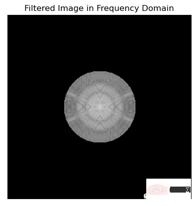
在可视化傅里叶频谱时，使用np.log(1+np.abs(x))和20*np.log(np.abs(x))之间的选择是个人喜好的问题，可以取决于具体的应用程序。

一般情况下会使用Np.log (1+np.abs(x))，因为它通过压缩数据的动态范围来帮助更清晰地可视化频谱。这是通过取数据绝对值的对数来实现的，并加上1以避免取零的对数。

而20*np.log(np.abs(x))将数据按20倍缩放，并对数据的绝对值取对数，这可以更容易地看到不同频率之间较小的幅度差异。但是它不会像np.log(1+np.abs(x))那样压缩数据的动态范围。

这两种方法都有各自的优点和缺点，最终取决于具体的应用程序和个人偏好。

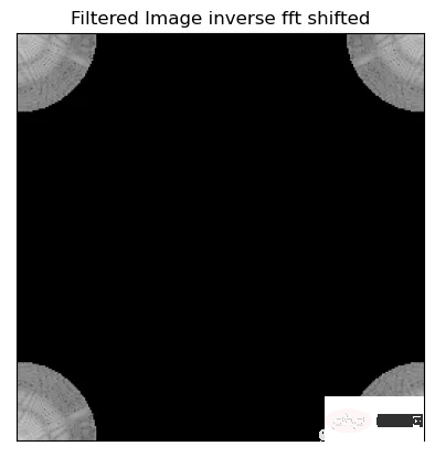
5、逆FFT位移

在频域滤波后，我们需要将图像移回原始位置，然后应用逆FFT。为了实现这一点，需要使用逆FFT移位，它反转了前面执行的移位过程。

fig, ax = plt.subplots()
 im = ax.imshow(np.log(1+np.abs(np.fft.ifftshift(fftshifted_image * idealFilterLP(50,img.shape)))), cmap='gray')
 ax.set_title('Filtered Image inverse fft shifted')
 ax.set_xticks([])
 ax.set_yticks([])
 
 fig.savefig('filtered image inverse fft shifted.png', bbox_inches='tight')

6、快速傅里叶逆变换(IFFT)

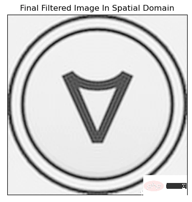
快速傅里叶逆变换(IFFT)是图像频率变换的最后一步。它用于将图像从频域传输回空间域。这一步的结果是在空间域中与原始图像相比，图像减少了噪声并提高了清晰度。

fig, ax = plt.subplots()
 im = ax.imshow(np.log(1+np.abs(np.fft.ifft2(np.fft.ifftshift(fftshifted_image * idealFilterLP(50,img.shape))))), cmap='gray')
 ax.set_title('Final Filtered Image In Spatial Domain')
 ax.set_xticks([])
 ax.set_yticks([])
 
 fig.savefig('final filtered image.png', bbox_inches='tight')

总结

我们再把所有的操作串在一起显示，

函数绘制所有图像

def Freq_Trans(image, filter_used):
 img_in_freq_domain = np.fft.fft2(image)
 
 # Shift the zero-frequency component to the center of the frequency spectrum
 centered = np.fft.fftshift(img_in_freq_domain)
 
 # Multiply the filter with the centered spectrum
 filtered_image_in_freq_domain = centered * filter_used
 
 # Shift the zero-frequency component back to the top-left corner of the frequency spectrum
 inverse_fftshift_on_filtered_image = np.fft.ifftshift(filtered_image_in_freq_domain)
 
 # Apply the inverse Fourier transform to obtain the final filtered image
 final_filtered_image = np.fft.ifft2(inverse_fftshift_on_filtered_image)
 
 return img_in_freq_domain,centered,filter_used,filtered_image_in_freq_domain,inverse_fftshift_on_filtered_image,final_filtered_image

使用高通、低通理想滤波器和高斯滤波器的直径分别为50、100和150像素，展示它们对增强图像清晰度的影响。

fig, axs = plt.subplots(12, 7, figsize=(30, 60))
 
 filters = [(f, d) for f in [idealFilterLP, idealFilterHP, gaussianLP, gaussianHP] for d in [50, 100, 150]]
 
 for row, (filter_name, filter_diameter) in enumerate(filters):
 # Plot each filter output on a separate subplot
 result = Freq_Trans(img, filter_name(filter_diameter, img.shape))
 
 for col, title, img_array in zip(range(7),
["Original Image", "Spectrum", "Centered Spectrum", f"{filter_name.__name__} of Diameter {filter_diameter} px",
 f"Centered Spectrum multiplied by {filter_name.__name__}", "Decentralize", "Processed Image"],
[img, np.log(1+np.abs(result[0])), np.log(1+np.abs(result[1])), np.abs(result[2]), np.log(1+np.abs(result[3])),
np.log(1+np.abs(result[4])), np.abs(result[5])]):
 
 axs[row, col].imshow(img_array, cmap='gray')
 axs[row, col].set_title(title)
 
 plt.tight_layout()
 plt.savefig('all_processess.png', bbox_inches='tight')
 plt.show()

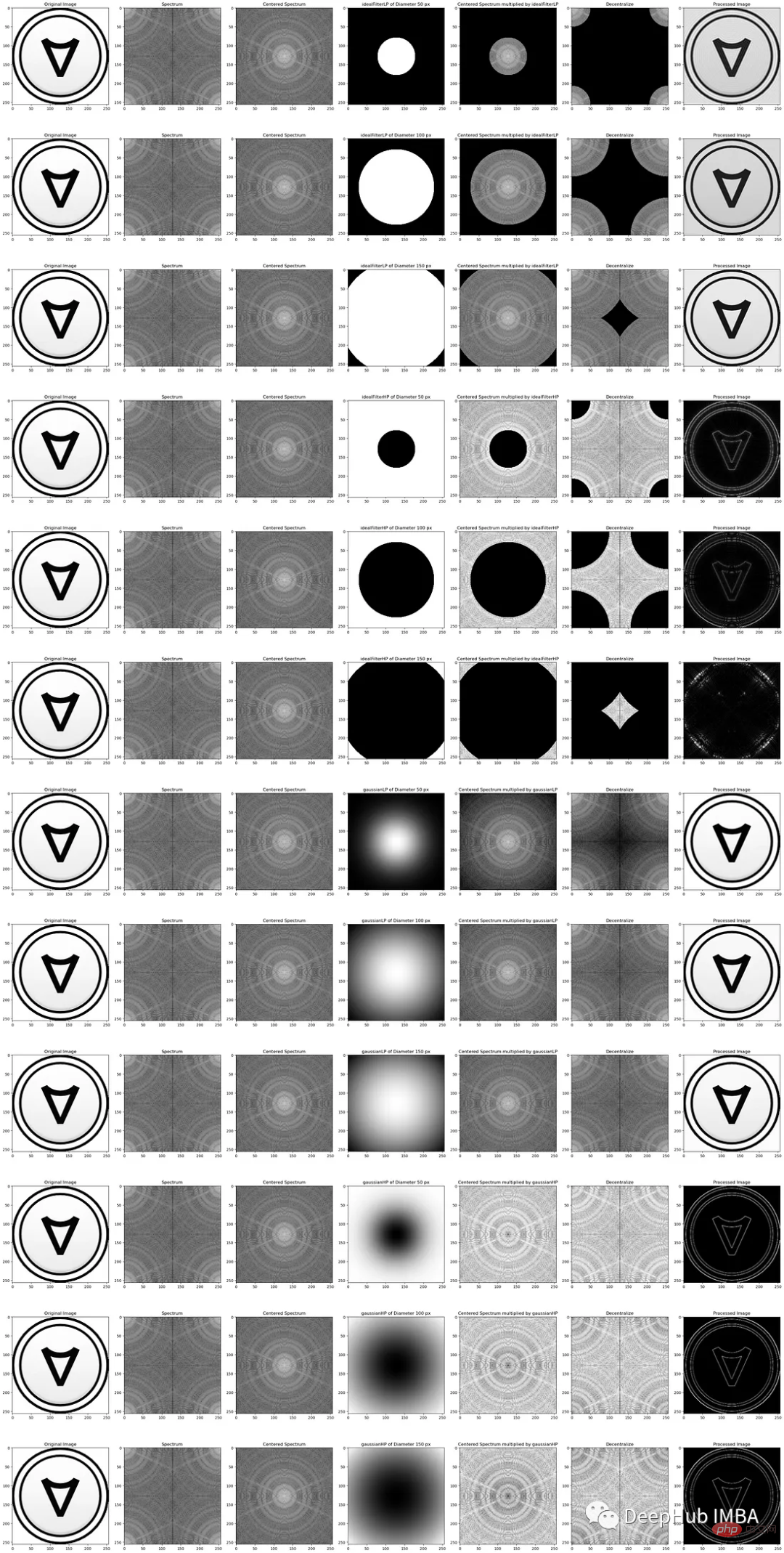
It can be seen that when changing the diameter of the circular mask, the impact on image clarity will be different. As the diameter increases, more frequencies are suppressed, resulting in smoother images with less detail. Reducing the diameter allows more frequencies to pass through, resulting in sharper images and more detail. In order to achieve the desired effect, it is important to choose the right diameter, as using a diameter that is too small will result in a filter that is not effective enough, while using a diameter that is too large will result in too much detail being lost.

Generally speaking, Gaussian filter is more commonly used in image processing tasks due to its smoothness and robustness. In some applications, where a sharper cutoff is required, an ideal filter may be more suitable.

Using FFT to modify the image frequency is an effective method to reduce noise and improve image sharpness. This involves using an FFT to convert the image to the frequency domain, using appropriate techniques to filter the noise, and using an inverse FFT to convert the modified image back to the spatial domain. By understanding and implementing these techniques, we can improve image quality for a variety of applications.

The above is the detailed content of Python image processing: frequency domain filtering, noise reduction and image enhancement. For more information, please follow other related articles on the PHP Chinese website!