Use Python to make a house price prediction gadget!

Hello, everyone.

This is a case of housing price prediction, which comes from the Kaggle website. It is the first competition question for many algorithm beginners.

This case has a complete process for solving machine learning problems, including EDA, feature engineering, model training, model fusion, etc.

House Price Prediction Process

Follow me and learn about this case.

No long words, no redundant code, just simple explanations.

1. EDA

The purpose of Exploratory Data Analysis (EDA) is to give us a full understanding of the data set. At this step, the content we explore is as follows:

##EDA content

1.1 Input data set

train = pd.read_csv('./data/train.csv')
test = pd.read_csv('./data/test.csv')

Training samples

train and test are training sets and test sets respectively, with 1460 samples and 80 features respectively.

The SalePrice column represents the housing price, which we want to predict.

1.2 House price distribution

Because our task is to predict house prices, the core thing to focus on in the data set is the value distribution of the house price (SalePrice) column.

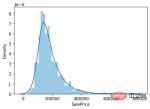
sns.distplot(train['SalePrice']);

House price value distribution

As can be seen from the figure, the peak value of the SalePrice column is relatively steep, and the peak value is skewed to the left.

You can also directly call the skew() and kurt() functions to calculate the specific skewness and kurtosis values ​​of SalePrice.

For situations where the skewness and kurtosis are relatively large, it is recommended to smooth the SalePrice column using log().

1.3 Features related to house prices

After understanding the distribution of SalePrice, we can calculate the correlation between 80 features and SalePrice.

Focus on the 10 features that are most relevant to SalePrice.

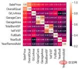
# 计算列之间相关性
corrmat = train.corr()
# 取 top10
k = 10
cols = corrmat.nlargest(k, 'SalePrice')['SalePrice'].index
# 绘图
cm = np.corrcoef(train[cols].values.T)
sns.set(font_scale=1.25)
hm = sns.heatmap(cm, cbar=True, annot=True, square=True, fmt='.2f', annot_kws={'size': 10}, yticklabels=cols.values, xticklabels=cols.values)
plt.show()

Features highly relevant to SalePrice

OverallQual (house materials and finishes), GrLivArea (above ground living area), GarageCars (garage capacity), and TotalBsmtSF (basement area) has a strong correlation with SalePrice.

These features will also be focused on when doing feature engineering later.

1.4 Eliminate outlier samples

Since the sample size of the data set is very small, outliers are not conducive to our subsequent training of the model.

So it is necessary to calculate the outliers of each numerical characteristic and eliminate the samples with the most outliers.

# 获取数值型特征
numeric_features = train.dtypes[train.dtypes != 'object'].index
# 计算每个特征的离群样本
for feature in numeric_features:
outs = detect_outliers(train[feature], train['SalePrice'],top=5, plot=False)
all_outliers.extend(outs)
# 输出离群次数最多的样本
print(Counter(all_outliers).most_common())
# 剔除离群样本
train = train.drop(train.index[outliers])

detect_outliers() is a custom function that uses the LocalOutlierFactor algorithm of the sklearn library to calculate outliers.

At this point, EDA is completed. Finally, the training set and test set are merged to perform the following feature engineering.

y = train.SalePrice.reset_index(drop=True)
train_features = train.drop(['SalePrice'], axis=1)
test_features = test
features = pd.concat([train_features, test_features]).reset_index(drop=True)

Features combines the features of the training set and the test set, which is the data we will process below.

2. Feature Engineering

##Feature Engineering

2.1 Correction feature type

MSSubClass (house type), YrSold (Sales year) and MoSold (Sales month) are categorical features, but they are represented by numbers, and they need to be converted into text features.

features['MSSubClass'] = features['MSSubClass'].apply(str)
features['YrSold'] = features['YrSold'].astype(str)
features['MoSold'] = features['MoSold'].astype(str)

2.2 Filling missing values ​​in features

There is no unified standard for filling missing values. It is necessary to decide how to fill in based on different features.

# Functional：文档提供了典型值 Typ
features['Functional'] = features['Functional'].fillna('Typ') #Typ 是典型值
# 分组填充需要按照相似的特征分组，取众数或中位数
# MSZoning（房屋区域）按照 MSSubClass（房屋）类型分组填充众数
features['MSZoning'] = features.groupby('MSSubClass')['MSZoning'].transform(lambda x: x.fillna(x.mode()[0]))
#LotFrontage（到接到举例）按Neighborhood分组填充中位数
features['LotFrontage'] = features.groupby('Neighborhood')['LotFrontage'].transform(lambda x: x.fillna(x.median()))
# 车库相关的数值型特征，空代表无，使用0填充空值。
for col in ('GarageYrBlt', 'GarageArea', 'GarageCars'):
features[col] = features[col].fillna(0)

2.3 Skewness Correction

Similar to exploring the SalePrice column, features with high skewness are smoothed.

# skew()方法，计算特征的偏度（skewness）。
skew_features = features[numeric_features].apply(lambda x: skew(x)).sort_values(ascending=False)
# 取偏度大于 0.15 的特征
high_skew = skew_features[skew_features > 0.15]
skew_index = high_skew.index
# 处理高偏度特征，将其转化为正态分布，也可以使用简单的log变换
for i in skew_index:
features[i] = boxcox1p(features[i], boxcox_normmax(features[i] + 1))

2.4 Feature deletion and addition

Features that are almost all missing values ​​or have a high proportion of single values ​​(99.94%) can be deleted directly.

features = features.drop(['Utilities', 'Street', 'PoolQC',], axis=1)

At the same time, multiple features can be fused to generate new features.

Sometimes it is difficult for the model to learn the relationship between features. Manual fusion of features can reduce the learning difficulty of the model and improve the effect.

# 将原施工日期和改造日期融合
features['YrBltAndRemod']=features['YearBuilt']+features['YearRemodAdd']
# 将地下室面积、1楼、2楼面积融合
features['TotalSF']=features['TotalBsmtSF'] + features['1stFlrSF'] + features['2ndFlrSF']

It can be found that the features we fuse are all features that are strongly related to SalePrice.

Finally simplify the features, and perform 01 processing on features with monotonous distribution (for example: 99 out of 100 data have a value of 0.9, and the other one has a value of 0.1).

features['haspool'] = features['PoolArea'].apply(lambda x: 1 if x > 0 else 0)
features['has2ndfloor'] = features['2ndFlrSF'].apply(lambda x: 1 if x > 0 else 0)

2.6 生成最终训练数据

到这里特征工程就做完了， 我们需要从features中将训练集和测试集重新分离出来，构造最终的训练数据。

X = features.iloc[:len(y), :]
X_sub = features.iloc[len(y):, :]
X = np.array(X.copy())
y = np.array(y)
X_sub = np.array(X_sub.copy())

三. 模型训练

因为SalePrice是数值型且是连续的，所以需要训练一个回归模型。

3.1 单一模型

首先以岭回归（Ridge） 为例，构造一个k折交叉验证模型。

from sklearn.linear_model import RidgeCV
from sklearn.pipeline import make_pipeline
from sklearn.model_selection import KFold
kfolds = KFold(n_splits=10, shuffle=True, random_state=42)
alphas_alt = [14.5, 14.6, 14.7, 14.8, 14.9, 15, 15.1, 15.2, 15.3, 15.4, 15.5]
ridge = make_pipeline(RobustScaler(), RidgeCV(alphas=alphas_alt, cv=kfolds))

岭回归模型有一个超参数alpha，而RidgeCV的参数名是alphas，代表输入一个超参数alpha数组。在拟合模型时，会从alpha数组中选择表现较好某个取值。

由于现在只有一个模型，无法确定岭回归是不是最佳模型。所以我们可以找一些出场率高的模型多试试。

# lasso
lasso = make_pipeline(
RobustScaler(),
LassoCV(max_iter=1e7, alphas=alphas2, random_state=42, cv=kfolds))
#elastic net
elasticnet = make_pipeline(
RobustScaler(),
ElasticNetCV(max_iter=1e7, alphas=e_alphas, cv=kfolds, l1_ratio=e_l1ratio))
#svm
svr = make_pipeline(RobustScaler(), SVR(
C=20,
epsilon=0.008,
gamma=0.0003,
))
#GradientBoosting（展开到一阶导数）
gbr = GradientBoostingRegressor(...)
#lightgbm
lightgbm = LGBMRegressor(...)
#xgboost（展开到二阶导数）
xgboost = XGBRegressor(...)

有了多个模型，我们可以再定义一个得分函数，对模型评分。

#模型评分函数
def cv_rmse(model, X=X):
rmse = np.sqrt(-cross_val_score(model, X, y, scoring="neg_mean_squared_error", cv=kfolds))
return (rmse)

以岭回归为例，计算模型得分。

score = cv_rmse(ridge)
print("Ridge score: {:.4f} ({:.4f})n".format(score.mean(), score.std()), datetime.now(), ) #0.1024

运行其他模型发现得分都差不多。

这时候我们可以任选一个模型，拟合，预测，提交训练结果。还是以岭回归为例

# 训练模型
ridge.fit(X, y)
# 模型预测
submission.iloc[:,1] = np.floor(np.expm1(ridge.predict(X_sub)))
# 输出测试结果
submission = pd.read_csv("./data/sample_submission.csv")
submission.to_csv("submission_single.csv", index=False)

submission_single.csv是岭回归预测的房价，我们可以把这个结果上传到 Kaggle 网站查看结果的得分和排名。

3.2 模型融合-stacking

有时候为了发挥多个模型的作用，我们会将多个模型融合，这种方式又被称为集成学习。

stacking 是一种常见的集成学习方法。简单来说，它会定义个元模型，其他模型的输出作为元模型的输入特征，元模型的输出将作为最终的预测结果。

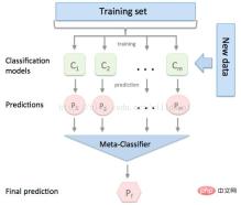
stacking

这里，我们用mlextend库中的StackingCVRegressor模块，对模型做stacking。

stack_gen =
StackingCVRegressor(
regressors=(ridge, lasso, elasticnet, gbr, xgboost, lightgbm),
meta_regressor=xgboost,
use_features_in_secondary=True)

训练、预测的过程与上面一样，这里不再赘述。

3.3 模型融合-线性融合

多模型线性融合的思想很简单，给每个模型分配一个权重（权重加和=1），最终的预测结果取各模型的加权平均值。

# 训练单个模型
ridge_model_full_data = ridge.fit(X, y)
lasso_model_full_data = lasso.fit(X, y)
elastic_model_full_data = elasticnet.fit(X, y)
gbr_model_full_data = gbr.fit(X, y)
xgb_model_full_data = xgboost.fit(X, y)
lgb_model_full_data = lightgbm.fit(X, y)
svr_model_full_data = svr.fit(X, y)
models = [
ridge_model_full_data, lasso_model_full_data, elastic_model_full_data,
gbr_model_full_data, xgb_model_full_data, lgb_model_full_data,
svr_model_full_data, stack_gen_model
]
# 分配模型权重
public_coefs = [0.1, 0.1, 0.1, 0.1, 0.15, 0.1, 0.1, 0.25]
# 线性融合，取加权平均
def linear_blend_models_predict(data_x,models,coefs, bias):
tmp=[model.predict(data_x) for model in models]
tmp = [c*d for c,d in zip(coefs,tmp)]
pres=np.array(tmp).swapaxes(0,1)
pres=np.sum(pres,axis=1)
return pres

到这里，房价预测的案例我们就讲解完了，大家可以自己运行一下，看看不同方式训练出来的模型效果。

回顾整个案例会发现，我们在数据预处理和特征工程上花费了很大心思，虽然机器学习问题模型原理比较难学，但实际过程中往往特征工程花费的心思最多。

The above is the detailed content of Use Python to make a house price prediction gadget!. For more information, please follow other related articles on the PHP Chinese website!