Practical Excel skills sharing: How to find the number one person with multiple criteria
- 青灯夜游forward
- 2023-03-07 18:43:405364browse
Ranking is simple; but if there are multiple project categories and there may be the same performance, how to quickly find out the person who ranks first in each share? This requires matching through multiple conditions to find the desired number one. There are two solutions provided here, but neither is perfect. Can you improve them?

#The annual commendation meeting is about to begin. Which colleagues will become the sales champions this year? Let's find them together!
The sales data of various types of electrical appliances on a company’s e-commerce platform is as shown in the figure:
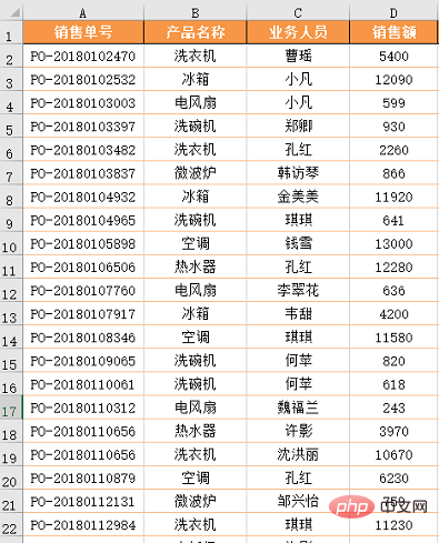
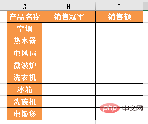
The data only has the sales order number, product name, business personnel name and sales volume , now it is necessary to count the sales champions of each type of product in the format shown below.
Seeing this problem, I wonder what methods you can think of? Pivot table, MAX function, or VLOOKUP...
The veteran recommends two methods: the first is the auxiliary column formula; the second is the pivot table formula.
Method 1: Auxiliary Column Formula
Step 1: Add Auxiliary Column
First Sum up each person's sales by product name. Sum according to conditions, here we use SUMIFS function for statistics. Although the same result can be achieved using a pivot table, the pivot table cannot obtain the final desired effect at once, so it is more convenient to use auxiliary columns.
Formula:
=SUMIFS(D:D,C:C,C2,B:B,B2)
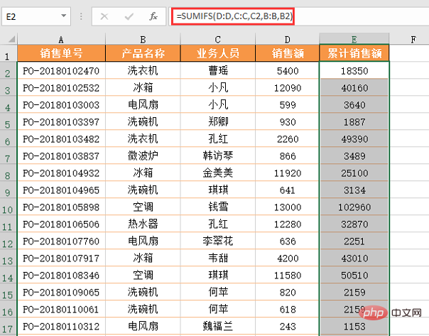
Formula format: =SUMIFS(summation area, condition area 1, condition 1, condition area 2, condition 2...)
SUMIFS is a multi-condition summation function , the first parameter is the column where the data to be summed is located, and the following parameters are grouped in pairs to form a set of conditions. In this example, the first set of conditions is business personnel, so condition area 1 is column C, condition 1 is C2; the second set of conditions is product name, condition area 2 is column B, and condition 2 is B2.
With the auxiliary column, the next step is to find out what the highest sales volume is in each category. What needs to be noted here is that in the statistical results table, the name of the sales champion comes first and the sales volume comes last. In actual statistics, it is not necessary to count in this order. We will count whichever is more convenient first.
Step 2: Statistics of the highest sales volume
Usually when talking about the maximum value, the first thing that comes to mind is the MAX function. The usage of this function is very similar to SUM. You only need to give a set of numbers or a data area to get the maximum value in this set of numbers.
In today’s example, because what we want to get is the maximum value in the same category, that is, the maximum value statistics based on conditions, we cannot directly use the MAX function to get the result.
This There is a fixed routine formula for counting the maximum value based on conditions:
=MAX(data area*(condition area 1=condition 1)*(condition area 2=condition 2)...)
This example has only one condition, which is the product name, so the formula is: =MAX($E$2:$E$750*($B$2:$B$750=G2))
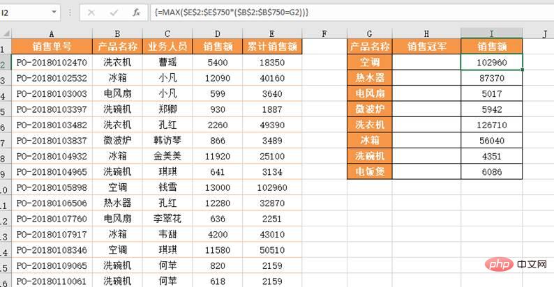
When using this formula, you need to pay attention to three things:
(1) The range must be accurate. It is not recommended to select the entire column as the calculation area;
(2) The formula involves array operations. After entering the formula, you need to press the Ctrl Shift Enter key. After pressing the key, a pair of curly brackets will be automatically added to the formula;
(3) Because the formula needs to be pulled down, in order to avoid The calculation area changes, so the involved range needs to use absolute references.
The specific principle of this formula involves the calculation principle of logical values and arrays, which we will explain specifically in the future.
At this point, find out the business personnel corresponding to the highest sales of each type of product and complete all statistics.
Step 3: Find the champion personnel
Check personnel based on sales, this is actually a search reference, use VLOOKUP or INDEX This can be done by other reference functions.
Nearly successful, now it’s time to peel the apple. The characteristic of peeling apples is thinness and accuracy.
The first detail: The cumulative sales in the data source are located to the right of the business person.
If we use VLOOKUP, we have to use the reverse search routine, and the formula is relatively complicated. It is possible to combine INDEX and MATCH, and the formula is not difficult:
=INDEX($C$2:$C$750,MATCH(I2,$E$2:$E$750,0))
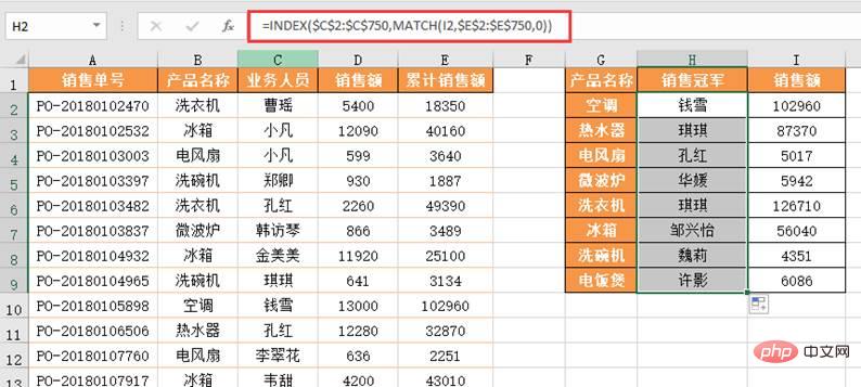
#The second detail: the maximum sales may be the same.
The combination of these two functions can be called a classic partner. But there is still a detail: we cannot rule out the possibility that the maximum sales of the two categories of products are the same. In order to avoid possible search errors when the maximum sales of different categories are the same, we must match based on the two conditions of product name and sales. The formula becomes:
=INDEX($C $2:$C$750,MATCH(G2&I2,$B$2:$B$750&$E$2:$E$750,0))
One of the common routines for multi-condition matching is to use the connection symbol & String multiple conditions together to form a new condition for query. Of course, the query area also needs to be strung together with &.
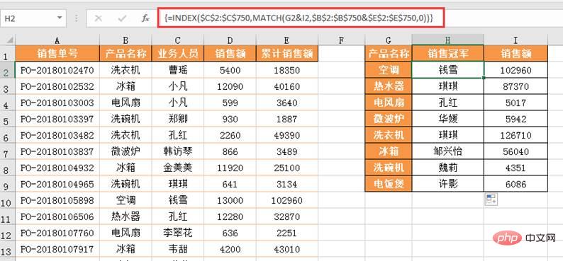
Of course, if you are looking for a multi-condition search like this and are unwilling to use Vlookup to reverse the search, you can also use the LOOKUP function to complete it:
=LOOKUP(1,0/(($E$2:$E$750=I2)*($B$2:$B$750=G2)),$C$2:$C$750)
The second common routine for multi-condition matching is to use the equal sign = to create an expression with the search area for multiple conditions, and then multiply the expressions.
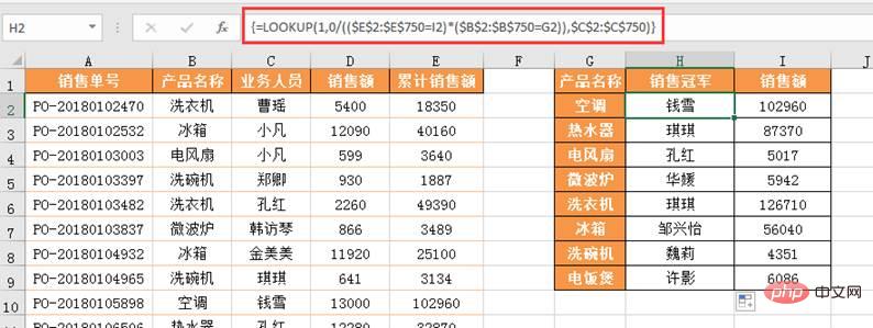
The formula is: =LOOKUP(1,0/(condition area=condition), target area), if there are multiple conditions , you can directly upgrade the routine to: =LOOKUP(1,0/((condition area 1=condition 1)*(condition area 2=condition 2)*(condition area 3=condition 3)..., target area )
Method 2: Pivot table formula
Step 1: Statistics and ranking
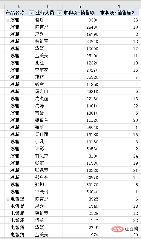
Drag the product name and business personnel into the row area, drag the sales volume twice to the value area, and then set sales volume 2 according to last year's tutorial from Tribe Nest Education "Hey, drag the mouse twice to get the performance statistics and rankings at once!" The value display mode is "descending order", and the basic field is "Business Personnel" to obtain sales performance statistics and rankings by product category.
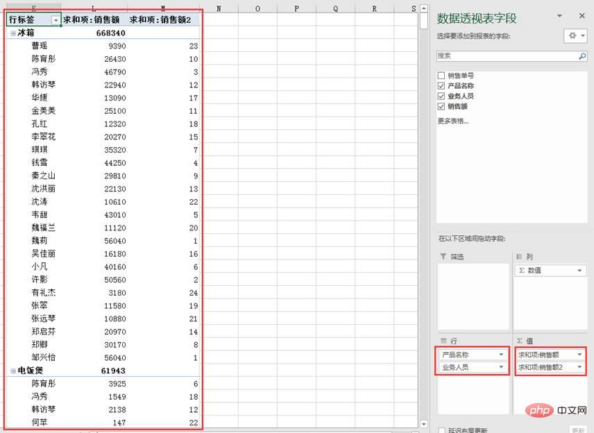
Step 2: Organize the pivot table
Click the pivot table and click "Display in table format" and "Display in table format" in the "Report Layout" drop-down menu in the "Layout" option group of the "Design" tab Repeat the "All Project Labels" command. Then right-click on the pivot table, select "Subtotal "Business Personnel"", and cancel the subtotal items in the table. The table becomes as follows:
Step 3, enter the formula to get the name and performance of the champion
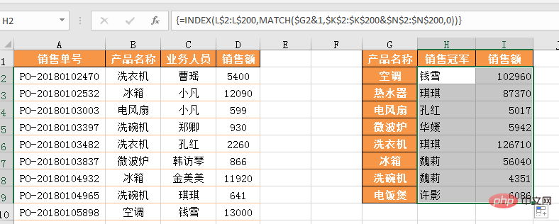
Enter the formula in cell G2:
=INDEX(L$2:L$200,MATCH($G2&1,$K$2:$K$200&$N$2:$N$200,0))
After inputting, press Ctrl Shift Enter three keys End.

Then right-click and pull-down the formula.
In today’s tutorial we learned a few functions, namely SUMIFS, MAX, INDEX, MATCH, and LOOKUP. I also learned two routines for multi-condition matching, which can be used directly when encountering similar problems.
However, today’s solution is Imperfect. Although we asked ourselves to "pee the apple" and pay attention to details in the tutorial, we still missed a very important detail - the highest sales of similar products may be the same.
Related learning recommendations: exceltutorial
The above is the detailed content of Practical Excel skills sharing: How to find the number one person with multiple criteria. For more information, please follow other related articles on the PHP Chinese website!
Related articles
See more- Practical Excel skills sharing: various ways to play format brush!
- Practical Excel skills sharing: 8 typical forms and problems of table headers
- Practical Excel skills sharing: common usage sharing of the 12 F keys (F1~F12)
- Detailed explanation of PHP using xlswriter to optimize Excel export performance (with code examples)
- Practical Excel skills sharing: 3 ways to quickly extract cell data
- Practical Excel Tips Sharing: Solutions to Common Printing Difficulties

