


I didn’t learn much about functions, so I focused on pivot tables. Pivot tables don’t disappoint, there are always little things that can solve big statistical problems. The 4 home remedies here are just that.

The so-called folk remedies refer to prescriptions that are rarely seen in normal times but have special effects on specific situations. Today we share with you 4 "recipes" for pivot tables.
Recipe 1: Null value processing
When we perform data pivot on a set of data, we often encounter the situation where the corresponding data of a certain field in the value area is blank. . In the past, many partners made manual modifications. In fact, you can customize the blank display to 0 through a pivot table. (Note: Only for blanks in the value area!)
Example:
The purchase quantity of the screen 300*220 item in the first quarter is blank, and now the data needs to be pivoted and summarized.

After completing the pivot, we see that cell C13 is blank.
Click the PivotTable, right-click the mouse, and select [PivotTable Options].

Open the [Pivot Table Options] dialog box, check [Display for blank cells] in [Layout and Format], and at the same time, in the edit bar on the right Enter "No data" in the box.

#After clicking OK, all the blank spaces in the PivotTable will be filled with "No Data" characters.

Note: Here we can fill the blanks with any text, numbers or symbols by definition.
Recipe 2: Ranking
In daily work, it is often necessary to rank the data after completing the data pivot. Many partners use the rank function to rank. In fact, pivot tables come with a ranking function, so there is no need for sorting or functions at all.
Still taking purchasing data as an example, now we have completed the data pivot.

Select the pivot table, right-click the mouse, select [Value Display Mode], and select [Sort Descending] in the submenu.

Select items as the basic field for sorting and click [OK].

Finally we saw that the original purchase data information turned into ranking information.

If we need to retain purchase data and ranking information at the same time, we only need to add the purchase quantity in the value field again.

Recipe Three: Create Worksheets in Batch
Batch creation is a task that is often encountered in daily life, such as creating branches, months , quarterly and other worksheets. If the number is small, we can create it one by one manually. What if the number is large? In fact, you can create worksheets in batches through pivot tables.
Example: Now we need to create a worksheet for 4 quarters.
First enter the header quarter and the names of the four quarters in the table.

Then select the data in column A and click [Pivot Table] in the [Insert] tab.
In the [Create PivotTable] dialog box that opens, select the location of the PivotTable as an existing worksheet.

After confirmation, drag the [Quarter] field to the filter box.

Click the PivotTable, and then click [Options] - [Show Report Filter Page] in the [Analysis] tab.

#The [Show Report Filter Page] dialog box appears, click OK directly, and we can see the batch-created worksheets.


Select all the worksheets created, then select the unnecessary data in the table in any worksheet, and select "Start" - " Clear"-"Clear All" to complete the batch creation of worksheets.

Is not it simple?
Note: Worksheets created in batches are automatically sorted by worksheet name. For example, for the first to fourth quarters here, the created worksheets are second, third, fourth, and first quarter in order. If you want to create a worksheet in quarterly order, change the input to Arabic numerals, such as the 1st, 2nd, 3rd, 4th, etc. quarters. If you want to create worksheets in the order of the names you enter, an easy way is to add Arabic numerals 1, 2, 3, etc. in front of each name when inputting, and the worksheets will be created in the order of input.
Recipe 4: Group statistics by new fields
It is also a common thing to group data by new fields for statistics. For example, there are no months or quarters in the data, but your boss asks you to make statistics on a monthly or quarterly basis; there are no first-, second-, or third-class products in the data, but your boss asks you to make statistics on first-, second-, and third-class products. For this kind of statistics of original data according to newly specified fields, it can be very easily implemented using a pivot table.
Give two examples.
Example 1: Group statistics by date
The data source is sales registered by day. Now we want to count sales by month and quarter.

(1) Select all the data and insert the pivot table.

(2) Drag the "Sales Date" field into the row area, Excel will automatically add a "Month" field (requires the 2016 version), and the row in the right pivot table Tags are displayed by month. (Note: If you are using an earlier version, you need to set the "Quarter" field as shown below. Only after adding the "Month" field can statistics be calculated on a monthly basis.) Then drag "Sales" into the value area.

(3) Next we implement quarterly statistics through grouping settings. Right-click on any data under the pivot table row label and select the "Combine" command (you can also click [Analyze] - [Group Field] or [Group Selection]) to open the [Combine] dialog box. You can see that the two step sizes "day" and "month" have been selected.

#Start at and end at data will be automatically generated based on the data source, don’t worry about it.
(4) Click "Quarter" and then OK.

# (5) You can see that the "Quarter" field has been added to the pivot table field. In the pivot table on the left, click the  symbol to collapse the data and achieve quarterly statistics.

Example 2: Score statistics by stages
The following table shows the mathematics scores of a certain class, with only two fields: name and score. . Now we need to count the number of people in each stage, 60-79, 80-100.

(1) Same as above, first create a pivot table.

(2) Drag the "Grade" field into the row area. At this time, a column of fractional values appears below the row labels of the left pivot table.

(3) Right-click on any score under the pivot table row label and select the "Combine" command to open the Combination dialog box.

# (4) Now modify the starting value, ending value, and step size as needed. The settings start at 60 and end at 100 in steps of 20, as follows.

(5) After clicking "OK", the row label changes to the three fractional segments we need.

(6) Drag the "Grade" field to the value area to implement headcount statistics. For example, there are 11 people who failed.
(7) If you want to further see the names at each stage, you can drag the "Name" field into the row area.
If you want to segment more freely without being restricted by the step size, you can change the approach in step (3). For example, select 0-59, right-click, select "Combine", generate "Data Group 1", select "Data Group 1", enter "D" in the edit bar, change "Data Group 1" to "D", this It is the grade D stage; select 60-79, right-click the combination and change it to "C"; select 80-90, right-click the combination and change it to "B"; select 90 or above, right-click the combination and change it to "A". In this way, the results are divided into four stages ABCD for statistics.

Summary:
Today I shared with you 4 practical "recipes" for pivot table functions. These folk remedies are very efficient and can replace complex function work and improve efficiency. If you pay more attention to some functions and options in your daily work, and think more, you will find one more skill to make Excel run more freely.
Related learning recommendations: excel tutorial
The above is the detailed content of The 4 most practical pivot table tips for learning Excel pivot tables. For more information, please follow other related articles on the PHP Chinese website!

 MEDIAN formula in Excel - practical examplesApr 11, 2025 pm 12:08 PM
This tutorial explains how to calculate the median of numerical data in Excel using the MEDIAN function. The median, a key measure of central tendency, identifies the middle value in a dataset, offering a more robust representation of central tenden
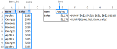
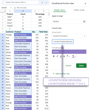 Google Spreadsheet COUNTIF function with formula examplesApr 11, 2025 pm 12:03 PM
Master Google Sheets COUNTIF: A Comprehensive Guide This guide explores the versatile COUNTIF function in Google Sheets, demonstrating its applications beyond simple cell counting. We'll cover various scenarios, from exact and partial matches to han
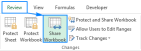 Excel shared workbook: How to share Excel file for multiple usersApr 11, 2025 am 11:58 AM
This tutorial provides a comprehensive guide to sharing Excel workbooks, covering various methods, access control, and conflict resolution. Modern Excel versions (2010, 2013, 2016, and later) simplify collaborative editing, eliminating the need to m
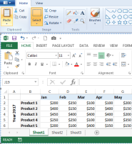 How to convert Excel to JPG - save .xls or .xlsx as image fileApr 11, 2025 am 11:31 AM
This tutorial explores various methods for converting .xls files to .jpg images, encompassing both built-in Windows tools and free online converters. Need to create a presentation, share spreadsheet data securely, or design a document? Converting yo
 Excel names and named ranges: how to define and use in formulasApr 11, 2025 am 11:13 AM
This tutorial clarifies the function of Excel names and demonstrates how to define names for cells, ranges, constants, or formulas. It also covers editing, filtering, and deleting defined names. Excel names, while incredibly useful, are often overlo
 Standard deviation Excel: functions and formula examplesApr 11, 2025 am 11:01 AM
This tutorial clarifies the distinction between standard deviation and standard error of the mean, guiding you on the optimal Excel functions for standard deviation calculations. In descriptive statistics, the mean and standard deviation are intrinsi
 Square root in Excel: SQRT function and other waysApr 11, 2025 am 10:34 AM
This Excel tutorial demonstrates how to calculate square roots and nth roots. Finding the square root is a common mathematical operation, and Excel offers several methods. Methods for Calculating Square Roots in Excel: Using the SQRT Function: The
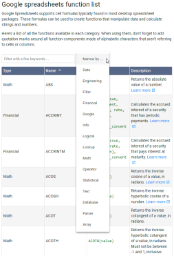 Google Sheets basics: Learn how to work with Google SpreadsheetsApr 11, 2025 am 10:23 AM
Unlock the Power of Google Sheets: A Beginner's Guide This tutorial introduces the fundamentals of Google Sheets, a powerful and versatile alternative to MS Excel. Learn how to effortlessly manage spreadsheets, leverage key features, and collaborate


Hot AI Tools

Undresser.AI Undress
AI-powered app for creating realistic nude photos

AI Clothes Remover
Online AI tool for removing clothes from photos.

Undress AI Tool
Undress images for free

Clothoff.io
AI clothes remover

Video Face Swap
Swap faces in any video effortlessly with our completely free AI face swap tool!

Hot Article
Hot Tools

PhpStorm Mac version
The latest (2018.2.1) professional PHP integrated development tool

MinGW - Minimalist GNU for Windows
This project is in the process of being migrated to osdn.net/projects/mingw, you can continue to follow us there. MinGW: A native Windows port of the GNU Compiler Collection (GCC), freely distributable import libraries and header files for building native Windows applications; includes extensions to the MSVC runtime to support C99 functionality. All MinGW software can run on 64-bit Windows platforms.

EditPlus Chinese cracked version
Small size, syntax highlighting, does not support code prompt function

DVWA
Damn Vulnerable Web App (DVWA) is a PHP/MySQL web application that is very vulnerable. Its main goals are to be an aid for security professionals to test their skills and tools in a legal environment, to help web developers better understand the process of securing web applications, and to help teachers/students teach/learn in a classroom environment Web application security. The goal of DVWA is to practice some of the most common web vulnerabilities through a simple and straightforward interface, with varying degrees of difficulty. Please note that this software

ZendStudio 13.5.1 Mac
Powerful PHP integrated development environment

