Excel cross-table extraction, Microsoft Query KO all functions
- 青灯夜游forward
- 2023-02-10 19:23:395480browse
Extracting data across tables The first reaction of many partners is functions such as VLOOKUP, or some INDEX SMALL IF formula. In fact, if you are extracting multiple columns of data, Microsoft Query, which has been left in the corner by many people for a long time, is the king! Not only is it easy to operate and easily solve "one-to-many" problems, but the result table it generates can form a dynamic link with the data source. If the data source changes, the results will be dynamically updated!

Today I would like to share with you a function that is rarely used but has miraculous effects---Microsoft Query to help you solve the "one-to-many" data extraction of two tables. Or to solve the problem of using one table to match another table to generate specific data.
As shown in the figure below, there are two worksheets in the same workbook. The "Department Personnel Information Table" lists the names of employees in each department and the corresponding supervisors, and the "Provincial Sales Data Table" lists The multiple provinces each employee is responsible for and the three-month sales data of the corresponding provinces. Now it is required to summarize the two tables into one table based on the name column.

Original table

Required results
How to use Microsoft Query?
STEP 01 Enable Microsoft Query and load data
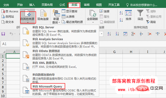
(1) Create a new workbook and click Under the [Data] tab, in the [Get External Data] group, select "From Microsoft" in the "From Other Sources" drop-down menu. Query".
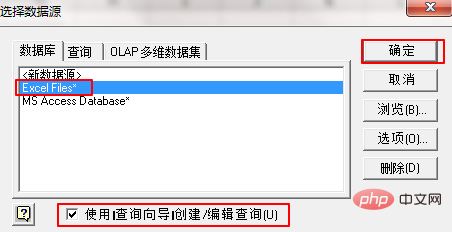
Click "Excel Files" under the "Database" option in the [Select Data Source] window, and check the box below "Use [Query Wizard] to create/edit queries ” and click OK.
Find the location of the data source in the directory on the right side of the [Select Workbook] window, find the file in the database name on the left, and click OK.

(2) Sometimes the system will prompt the following window: "The data source does not contain visible tables." Ignore this and click OK.

Enter the [Query Wizard] window on the left below, click the "Options" button below, open the [Table Options] window on the right, check "System Table" and click OK.

In this way, the worksheet in the data source will appear in the [Query Wizard] window. This is because Excel calls its own worksheet "system table". After checking it, you can See it.

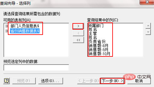
Next, select the two worksheets and click the ">" button in the middle to add the "Available tables and columns" on the left to the right "Query the columns in the results" and click Next.
Another window will pop up, prompting "The "Query Wizard" cannot continue because the table cannot be linked to Your query is in progress. You must be at Microsoft Drag fields between tables in Query to manually link. "Don't worry about this, click OK.

STEP 02 Match data as required
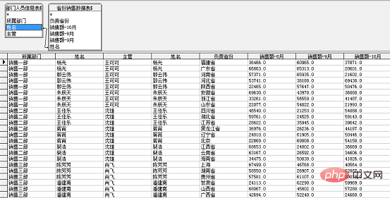
At this point we enter the Microsoft Query window. The top is a menu bar similar to EXCEL, and the middle is the table area, which displays the two tables we have added and the corresponding fields. The data area below is a fusion of the two The results of the table.
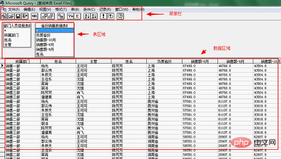
At this time, the results of the data area are messy. The reason is that we have not added a relationship to the two tables. The two tables are separated by the name column. One corresponding.
(1) Use the mouse to select the "Name" in the "Department Personnel Information Table" on the left, drag it to the "Name" in the "Provincial Sales Data Table" in the right table, and then release the mouse. At this time, a connecting line with small nodes at both ends appears between the "name" fields of the two tables. The data area below is updated immediately.
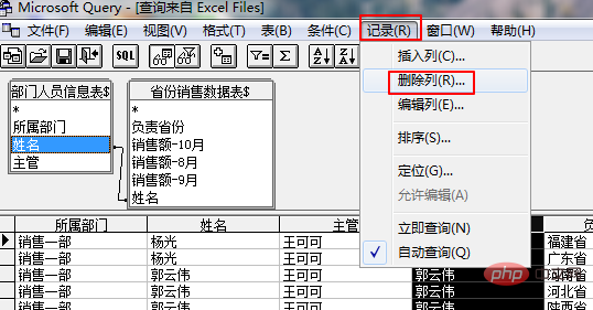
(2) Since there are two columns of the same name, we select one of the columns and click "Delete Column" under [Record] in the menu bar.
STEP 03 Return the result data to the Excel worksheet
Finally All you have to do is return the results to EXCEL.
(1) Click the button on the left side of "SQL" in the menu bar to return the data to Excel.

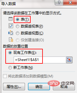
(2) The [Import Data] window appears in EXCEL. We choose to display it as "Table" and place it in the existing worksheet.
The return result is as follows:

In these simple 3 steps, we have completed the required data matching and generated New datasheet.
Extra joy
We found that the data generated by Microsoft Query is a super table, and you can also directly create a pivot table or pivot chart.
At the same time, this table is dynamically linked to the data source. For example, if we modify the original data, click Save to close.

Right-click on the returned results to refresh.

The data will be synchronized.

Application conditions
It should be noted that when using this method, the standardization of the data source must be ensured. It is required that the worksheet cannot contain data unrelated to the data source, and the first line of the table must be column headers. If you want to implement dynamic linking, the names and locations of the workbook and worksheet cannot be modified.
How is it, have you learned it? Is it simpler than PQ or simpler than a function?
Related learning recommendations: excel tutorial
The above is the detailed content of Excel cross-table extraction, Microsoft Query KO all functions. For more information, please follow other related articles on the PHP Chinese website!
Related articles
See more- Practical Excel skills sharing: examples of using shortcut keys [Ctrl+E]
- Excel function learning: CHOOSE function vs IF function
- Practical Excel skills sharing: two ways to quickly split a worksheet
- Practical Excel skills sharing: 7 practical positioning skills to help you improve work efficiency
- Sharing useful information: How to convert Word and Excel documents to each other
- Excel table collaboration: share workbooks and create a table with colleagues!
- Excel chart learning: making a combination of line chart and column chart

