
Home >Java >javaTutorial >Detailed graphic explanation of Java data structures and algorithms
Detailed graphic explanation of Java data structures and algorithms

- WBOYWBOYWBOYWBOYWBOYWBOYWBOYWBOYWBOYWBOYWBOYWBOYWBforward
- 2022-03-21 17:35:112439browse
This article brings you relevant knowledge about java, which mainly introduces java code implementation, annotation analysis, algorithm analysis and other related issues. I hope the detailed explanations in pictures and texts will be helpful to everyone.

java Learning Tutorial"
Chapter 1 Overview of Data Structure and Algorithm Basics 1.1 The importance of data structures and algorithms- ##Algorithms are the soul of programs. Excellent programs can still maintain high-speed calculations when calculating massive amounts of data
- The relationship between data structure and algorithm
:
Program = data structure algorithm- The data structure is the basis of the algorithm, in other words, If you want to learn algorithms well, you need to know the data structure well.
- Data structure and algorithm learning outline
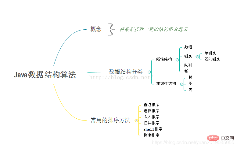 1.2 Data structure overview
 Logical structure
- Set structure
- : Data elements belong to the same set, and they are juxtaposed Relationship, no other relationship; it can be understood as a collection of learning in middle school. Within a range, there are many elements, and there is no relationship between elements. Linear structure
- : between elements There is a one-to-one relationship; it can be understood that each student corresponds to a student number, and the student number and name are linear structures Tree structure
- : There is a pair between elements The relationship of many can be simply understood as a family genealogy, one generation after another. Graphic structure
- : There is a many-to-many relationship between elements. Each element may correspond to multiple elements. Or corresponding to multiple elements, network graph Storage structure
- Sequential storage structure
- : It means to store data continuously, we can Compare it to queuing up for meals in a school cafeteria, one after another; Chained storage structure
- : It is not stored in order. The next number that comes in only needs to tell its address. The previous node, the address of the number behind it is stored in the previous node, so the storage address of the last number is null; this structure can be compared to calling a number at a shopping mall, and the number above is compared to an address. You What is the subsequent address? The other content above is the content of the node; Difference
- : The characteristic of sequential storage is that querying is fast and insertion or deletion is slow.
- The characteristics of chain storage are slow query and fast insertion or deletion
1.3 Algorithm Overview
- Judge the quality of the algorithm through time and space complexity
- There is no best algorithm, only the most appropriate. Learning algorithms is to accumulate learning ideas and master learning ideas, not to Solve a certain problem to remember a certain algorithm; regarding time complexity and space complexity, in most development situations now, we are using space for time, consuming more memory to ensure faster speed.
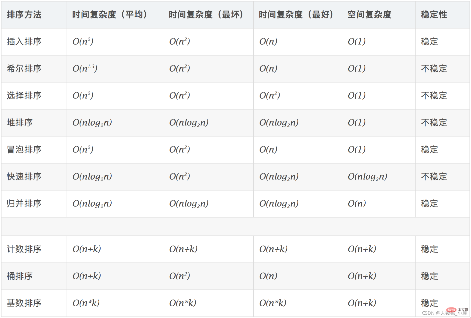
- Complexity and stability of each sorting algorithm
- :
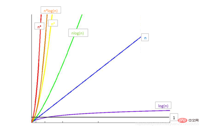
 How to understand "Big O notation"
Particularly specific and detailed analysis of algorithms, while great, has limited practical value in practice. For the temporal and spatial properties of the algorithm, the most important thing is its magnitude and trend, which are the main part of analyzing the efficiency of the algorithm. The constant factors in the size function that measure the number of basic operations of the algorithm can be ignored. For example, it can be considered that 3n^2 and 100n^2 belong to the same order of magnitude. If the cost of two algorithms processing instances of the same size is these two functions, their efficiency is considered to be "similar", and both are n^2 level.
Time complexity
The time an algorithm takes is proportional to the number of executions of statements in the algorithm. Which algorithm has more statements, it takes more time. The number of statement executions in the algorithm is called statement frequency or time frequency, recorded as
T(n). n is called the scale of the problem. When n continues to change, the time frequency Generally, the number of times the basic operations in the algorithm are repeated is a function of the problem size n, represented by Basic calculation rules for time complexity: common time complexity: Common The relationship between time complexity: Case 1: T(n) will also continue to change. But sometimes we want to know what pattern it shows when it changes. To this end, we introduce the concept of Time Complexity. T(n). If there is an auxiliary function f(n) , so that when n approaches infinitely large, the limit value of T(n)/f(n) is a constant not equal to zero, then it is called f(n) is a function of the same order of magnitude as T(n). Denoted as T(n)=O(f(n)), we call O(f(n)) the asymptotic time complexity of the algorithm, abbreviated as time complexity. Basic operations, that is, only constant terms, are considered to have a time complexity of O(1)

: Log2n (logarithm with base 2) is often abbreviated as logn
count = 0;				      (1)
	for(i = 0;i
- statement (1) executes 1
- statement (2) Execute the
- statement n times (3) Execute the
- statement n^2 times (4) Execute the
- statement n^2 times. The time complexity is : T(n) = 1 n n^2 n^2 = O(n^2)
: a = 1; (1)
b = 2; (2)
for(int i = 1;i
- Statement (3) is executed n times
- Statement (4), (5), (6) is executed n times
- The time complexity is
- : T(n) = 1 1 4n = o(n)
i = 1;		 (1)while(i<n i><strong></strong>The frequency of statement (1) is 1<ul>Suppose the frequency of statement (2) is<li>f(n)</li>, then <li>2f(n), take the maximum value f(n) = log2n<code></code><code></code>The time complexity is </li>:<li>T(n) = O(log2n)<strong></strong><code></code>Space complexity</li>
</ul>
<h3></h3>The space complexity calculation formula of the algorithm : <ul>S(n) = 0( f(n) )<li>, where n is the input size, <p>f(n)<code> is the function of the storage space occupied by n in the statement</code><code></code></p>The storage space occupied by an algorithm on the computer memory includes three aspects</li>
<li>
<p>The storage space occupied by the storage algorithm itself</p>
<ul>Input of the algorithm The storage space occupied by the output data<li>The storage space temporarily occupied by the algorithm during operation<li>
<li>
</ul>
</li>Case</ul>: The specified array is used Reverse and return the reversed content<p><strong>Solution 1:</strong></p>
<pre class="brush:php;toolbar:false">public static int[] reverse1(int[] arr) {
    int n = arr.length; //申请4个字节
    int temp; //申请4个字节
    for (int start = 0, end = n - 1; start <p></p>The space complexity is
- :
- S(n) = 4 4 = O(8) = O(1)
Solution 2:
public static int[] reverse2(int[] arr) {
    int n = arr.length; //申请4个字节
    int[] temp = new int[n]; //申请n*4个字节+数组自身头信息开销24个字节
    for (int i = n - 1; i >= 0; i--) {
        temp[n - 1 - i] = arr[i];
    }
    return temp;}
The space complexity is - :
- S( n) = 4 4n 24 = O(n 28) = O(n)
According to the big O derivation rule, the space complexity of algorithm one is 0(1), and that of algorithm two is The space complexity is 0(n), so from the perspective of space occupation, algorithm one is better than algorithm two.
Normal situation Let’s talk about the complexity directly. The default is the time complexity of the algorithm
.However, if the program you are doing is embedded development, especially the built-in program on some sensor devices, since the memory of these devices is very small, usually a few kb, the space complexity of the algorithm will be There are requirements, but generally those who do Java development are basically server development, and generally there is no such problem.
第2章 数组
2.1 数组概念
数组是一种线性表数据结构,它用一组连续的内存空间,来存储一组具有相同类型的数据。这里我们要抽取出三个跟数组相关的关键词:线性表,连续内存空间,相同数据类型;数组具有连续的内存空间,存储相同类型的数据,正是该特性使得数组具有一个特性:随机访问。但是有利有弊,这个特性虽然使得访问数组边得非常容易,但是也使得数组插入和删除操作会变得很低效,插入和删除数据后为了保证连续性,要做很多数据搬迁工作。
查找数组中的方法有两种:
- 线性查找:线性查找就是简单的查找数组中的元素
- 二分法查找:二分法查找要求目标数组必须是有序的。
2.2 无序数组
- 实现类:
public class MyArray {
	//声明一个数组
	private long[] arr;

	//有效数据的长度
	private int elements;

	//无参构造函数,默认长度为50
	public MyArray(){
		arr = new long[50];
	}

	public MyArray(int maxsize){
		arr = new long[maxsize];
	}


	//添加数据
	public void insert(long value){
		arr[elements] = value;
		elements++;
	}

	//显示数据
	public void display(){
		System.out.print("[");
		for(int i = 0;i = elements || index = elements || index = elements || index
-
优点:插入快(时间复杂度为:
O(1))、如果知道下标,可以很快存储 -
缺点:查询慢(时间复杂度为:
O(n))、删除慢
2.3 有序数组
- 实现类:
public class MyOrderArray {
	private long[] arr;

	private int elements;

	public MyOrderArray(){
		arr = new long[50];
	}

	public MyOrderArray(int maxsize){
		arr = new long[maxsize];
	}

	//添加数据
	public void insert(int value){
		int i;
		for(i = 0;i  value){
				break;
			}
		}
		for(int j = elements;j > i;j--){
			arr[j] = arr[j -1];
		}
		arr[i] = value;
		elements++;
	}


	//删除数据
	public void delete(int index){
		if(index >=elements || index = elements || index = elements || index  pow){
					return -1;
				}else{
					if(arr[middle] > value){
						//待查询的数在左边,右指针重新改变指向
						pow = middle-1;
					}else{
						//带查询的数在右边,左指针重新改变指向
						low = middle +1;
					}
				}
			}
	}}
-
优点:查询快(时间复杂度为:
O(logn)) -
缺点:增删慢(时间复杂度为:
O(n))
第三章 栈
3.1 栈概念
栈(stack),有些地方称为堆栈,是一种容器,可存入数据元素、访问元素、删除元素,它的特点在于只能允许在容器的一端(称为栈顶端指标,英语:top)进行加入数据(英语:push)和输出数据(英语:pop)的运算。没有了位置概念,保证任何时候可以访问、删除的元素都是此前最后存入的那个元素,确定了一种默认的访问顺序。
由于栈数据结构只允许在一端进行操作,因而按照后进先出的原理运作。
栈可以用顺序表实现,也可以用链表实现。

3.2 栈的操作
- Stack() 创建一个新的空栈
- push(element) 添加一个新的元素element到栈顶
- pop() 取出栈顶元素
- peek() 返回栈顶元素
- is_empty() 判断栈是否为空
- size() 返回栈的元素个数
实现类:
package mystack;public class MyStack {

    //栈的底层使用数组来存储数据
    //private int[] elements;
    int[] elements; //测试时使用

    public MyStack() {
        elements = new int[0];
    }

    //添加元素
    public void push(int element) {
        //创建一个新的数组
        int[] newArr = new int[elements.length + 1];
        //把原数组中的元素复制到新数组中
        for (int i = 0; i <p><strong>测试类</strong>:</p><pre class="brush:php;toolbar:false">package mystack;public class Demo {
    public static void main(String[] args) {
        MyStack ms = new MyStack();
        //添加元素
        ms.push(9);
        ms.push(8);
        ms.push(7);

        //取出栈顶元素//        System.out.println(ms.pop()); //7//        System.out.println(ms.pop()); //8//        System.out.println(ms.pop()); //9

        //查看栈顶元素
        System.out.println(ms.peek()); //7
        System.out.println(ms.peek()); //7

        //查看栈中元素个数
        System.out.println(ms.size()); //3
    }}
第4章 队列
4.1 队列概念
队列(Queue)是只允许在一端进行插入操作,而在另一端进行删除操作的线性表。
队列是一种先进先出的(First In First Out)的线性表,简称FIFO。允许插入的一端为队尾,允许删除的一端为队头。队列不允许在中间部位进行操作!假设队列是q=(a1,a2,……,an),那么a1就是队头元素,而an是队尾元素。这样我们就可以删除时,总是从a1开始,而插入时,总是在队列最后。这也比较符合我们通常生活中的习惯,排在第一个的优先出列,最后来的当然排在队伍最后。
同栈一样,队列也可以用顺序表或者链表实现。

4.2 队列的操作
- Queue() 创建一个空的队列
- enqueue(element) 往队列中添加一个element元素
- dequeue() 从队列头部删除一个元素
- is_empty() 判断一个队列是否为空
- size() 返回队列的大小
实现类:
public class MyQueue {

    int[] elements;

    public MyQueue() {
        elements = new int[0];
    }

    //入队
    public void enqueue(int element) {
        //创建一个新的数组
        int[] newArr = new int[elements.length + 1];
        //把原数组中的元素复制到新数组中
        for (int i = 0; i <p><strong>测试类</strong>:</p><pre class="brush:php;toolbar:false">public class Demo {
    public static void main(String[] args) {
        MyQueue mq = new MyQueue();

        //入队
        mq.enqueue(1);
        mq.enqueue(2);
        mq.enqueue(3);

        //出队
        System.out.println(mq.dequeue()); //1
        System.out.println(mq.dequeue()); //2
        System.out.println(mq.dequeue()); //3
    }}
第5章 链表
5.1 单链表
单链表概念
单链表也叫单向链表,是链表中最简单的一种形式,它的每个节点包含两个域,一个信息域(元素域)和一个链接域。这个链接指向链表中的下一个节点,而最后一个节点的链接域则指向一个空值。

- 表元素域data用来存放具体的数据。
- 链接域next用来存放下一个节点的位置
单链表操作
- is_empty() 链表是否为空
- length() 链表长度
- travel() 遍历整个链表
- add(item) 链表头部添加元素
- append(item) 链表尾部添加元素
- insert(pos, item) 指定位置添加元素
- remove(item) 删除节点
- search(item) 查找节点是否存在
实现类:
//一个节点public class Node {

    //节点内容
    int data;
    //下一个节点
    Node next;

    public Node(int data) {
        this.data = data;
    }

    //为节点追加节点
    public Node append(Node node) {
        //当前节点
        Node currentNode = this;
        //循环向后找
        while (true) {
            //取出下一个节点
            Node nextNode = currentNode.next();
            //如果下一个节点为null,当前节点已经是最后一个节点
            if (nextNode == null) {
                break;
            }
            //赋给当前节点,无线向后找
            currentNode = nextNode;
        }
        //把需要追加的节点,追加为找到的当前节点(最后一个节点)的下一个节点
        currentNode.next = node;
        return this;
    }

    //显示所有节点信息
    public void show() {
        Node currentNode = this;
        while (true) {
            System.out.print(currentNode.data + " ");
            //取出下一个节点
            currentNode = currentNode.next;
            //如果是最后一个节点
            if (currentNode == null) {
                break;
            }
        }
        System.out.println();
    }

    //插入一个节点作为当前节点的下一个节点
    public void after(Node node) {
        //取出下一个节点,作为下下一个节点
        Node nextNext = next;
        //把新节点作为当前节点的下一个节点
        this.next = node;
        //把下下一个节点设置为新节点的下一个节点
        node.next = nextNext;

    }

    //删除下一个节点
    public void removeNode() {
        //取出下下一个节点
        Node newNext = next.next;
        //把下下一个节点设置为当前节点的下一个节点
        this.next = newNext;
    }

    //获取下一个节点
    public Node next() {
        return this.next;
    }

    //获取节点中的数据
    public int getData() {
        return this.data;
    }

    //判断节点是否为最后一个节点
    public boolean isLast() {
        return next == null;
    }}
测试类:
public class Demo {
    public static void main(String[] args) {
        //创建节点
        Node n1 = new Node(1);
        Node n2 = new Node(2);
        Node n3 = new Node(3);
        //追加节点
        n1.append(n2).append(n3);
        //取出下一个节点数据
        System.out.println(n1.next().next().getData()); //3
        //判断节点是否为最后一个节点
        System.out.println(n1.isLast()); //false
        System.out.println(n1.next().next().isLast()); //true
        //显示所有节点信息
        n1.show(); //1 2 3
        //删除一个节点//        n1.next.removeNode();//        n1.show(); //1 2
        //插入一个新节点
        n1.next.after(new Node(0));
        n1.show(); //1 2 0 3
    }}
5.2 循环链表
循环链表概念
单链表的一个变形是单向循环链表,链表中最后一个节点的 next 域不再为 None,而是指向链表的头节点。
循环链表操作
实现类:
//表示一个节点public class LoopNode {

    //节点内容
    int data;
    //下一个节点
    LoopNode next = this; //与单链表的区别,追加了一个this,当只有一个节点时指向自己

    public LoopNode(int data) {
        this.data = data;
    }

    //插入一个节点
    public void after(LoopNode node) {
        LoopNode afterNode = this.next;
        this.next = node;
        node.next = afterNode;
    }

    //删除一个节点
    public void removeNext() {
        LoopNode newNode = this.next.next;
        this.next = newNode;
    }

    //获取下一个节点
    public LoopNode next() {
        return this.next;
    }

    //获取节点中的数据
    public int getData() {
        return this.data;
    }}
测试类:
public class Demo {
    public static void main(String[] args) {
        //创建节点
        LoopNode n1 = new LoopNode(1);
        LoopNode n2 = new LoopNode(2);
        LoopNode n3 = new LoopNode(3);
        LoopNode n4 = new LoopNode(4);

        //增加节点
        n1.after(n2);
        n2.after(n3);
        n3.after(n4);
        System.out.println(n1.next().getData()); //2
        System.out.println(n2.next().getData()); //3
        System.out.println(n3.next().getData()); //4
        System.out.println(n4.next().getData()); //1
    }}
5.3 双向循环链表
双向循环链表概念
在双向链表中有两个指针域,一个是指向前驱结点的prev,一个是指向后继结点的next指针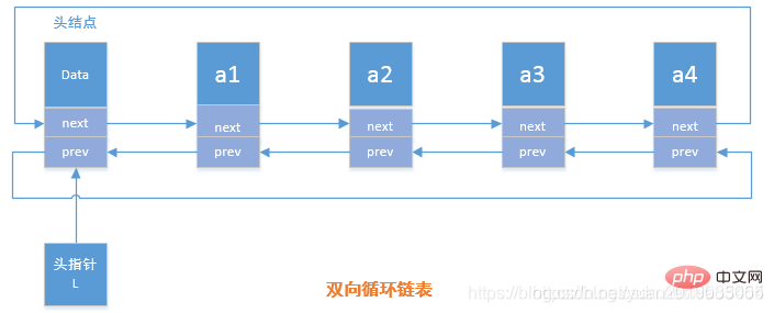
双向循环链表操作
实现类:
public class DoubleNode {
    //上一个节点
    DoubleNode pre = this;
    //下一个节点
    DoubleNode next = this;
    //节点数据
    int data;

    public DoubleNode(int data) {
        this.data = data;
    }

    //增加节点
    public void after(DoubleNode node) {
        //原来的下一个节点
        DoubleNode nextNext = next;
        //新节点作为当前节点的下一个节点
        this.next = node;
        //当前节点作为新节点的前一个节点
        node.pre = this;
        //原来的下一个节点作为新节点的下一个节点
        node.next = nextNext;
        //原来的下一个节点的上一个节点为新节点
        nextNext.pre = node;
    }

    //获取下一个节点
    public DoubleNode getNext() {
        return this.next;
    }

    //获取上一个节点
    public DoubleNode getPre() {
        return this.pre;
    }

    //获取数据
    public int getData() {
        return this.data;
    }}
测试类:
public class Demo {
    public static void main(String[] args) {
        //创建节点
        DoubleNode n1 = new DoubleNode(1);
        DoubleNode n2 = new DoubleNode(2);
        DoubleNode n3 = new DoubleNode(3);

        //追加节点
        n1.after(n2);
        n2.after(n3);

        //查看上一个,自己,下一个节点内容
        System.out.println(n2.getPre().getData()); //1
        System.out.println(n2.getData()); //2
        System.out.println(n2.getNext().getData()); //3

        System.out.println(n1.getPre().getData()); //3
        System.out.println(n3.getNext().getData()); //1
    }}
第6章 树结构基础
6.1 为什么要使用树结构
线性结构中不论是数组还是链表,他们都存在着诟病;比如查找某个数必须从头开始查,消耗较多的时间。使用树结构,在插入和查找的性能上相对都会比线性结构要好
6.2 树结构基本概念
示意图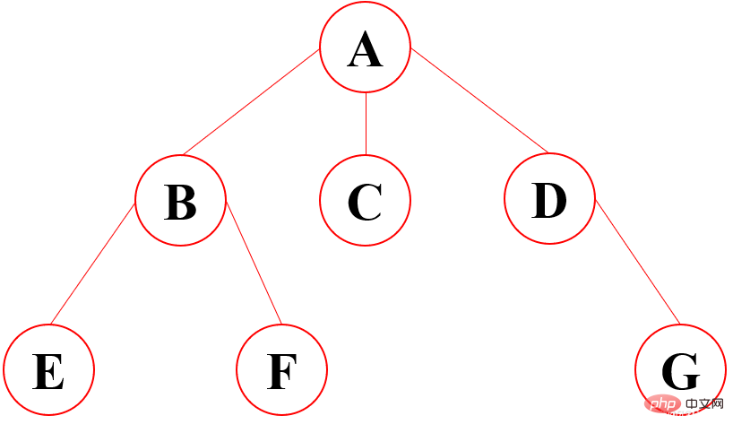
1、根节点:最顶上的唯一的一个;如:A
2、双亲节点:子节点的父节点就叫做双亲节点;如A是B、C、D的双亲节点,B是E、F的双亲节点
3、子节点:双亲节点所产生的节点就是子节点
4、路径:从根节点到目标节点所走的路程叫做路径;如A要访问F,路径为A-B-F
5、节点的度:有多少个子节点就有多少的度(最下面的度一定为0,所以是叶子节点)
6、节点的权:在节点中所存的数字
7、叶子节点:没有子节点的节点,就是没有下一代的节点;如:E、F、C、G
8、子树:在整棵树中将一部分看成也是一棵树,即使只有一个节点也是一棵树,不过这个树是在整个大树职中的,包含的关系
9、层:就是族谱中有多少代的人;如:A是1,B、C、D是2,E、F、G是3
10、树的高度:树的最大的层数:就是层数中的最大值
11、森林:多个树组成的集合
6.3 树的种类
无序树:树中任意节点的子节点之间没有顺序关系,这种树称为无序树,也称为自由树;
有序树:树中任意节点的子节点之间有顺序关系,这种树称为有序树;
-
二叉树:每个节点最多含有两个子树的树称为二叉树;
- 完全二叉树:对于一颗二叉树,假设其深度为d(d>1)。除了第d层外,其它各层的节点数目均已达最大值,且第d层所有节点从左向右连续地紧密排列,这样的二叉树被称为完全二叉树,其中满二叉树的定义是所有叶节点都在最底层的完全二叉树;
- 平衡二叉树(AVL树):当且仅当任何节点的两棵子树的高度差不大于1的二叉树;
- 排序二叉树(二叉查找树(英语:Binary Search Tree),也称二叉搜索树、有序二叉树);
- 霍夫曼树(用于信息编码):带权路径最短的二叉树称为哈夫曼树或最优二叉树;
- B树:一种对读写操作进行优化的自平衡的二叉查找树,能够保持数据有序,拥有多余两个子树。
6.4 树的存储与表示
顺序存储:将数据结构存储在固定的数组中,然在遍历速度上有一定的优势,但因所占空间比较大,是非主流二叉树。二叉树通常以链式存储。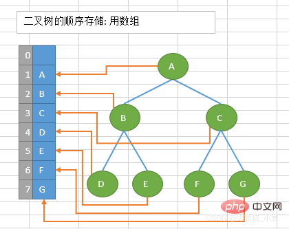
链式存储: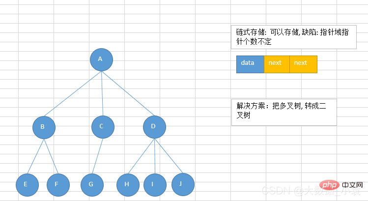
由于对节点的个数无法掌握,常见树的存储表示都转换成二叉树进行处理,子节点个数最多为2
6.5 常见的一些树的应用场景
1、xml,html等,那么编写这些东西的解析器的时候,不可避免用到树
2、路由协议就是使用了树的算法
3、mysql数据库索引
4、文件系统的目录结构
5、所以很多经典的AI算法其实都是树搜索,此外机器学习中的decision tree也是树结构
第7章 二叉树大全
7.1 二叉树的定义
任何一个节点的子节点数量不超过 2,那就是二叉树;二叉树的子节点分为左节点和右节点,不能颠倒位置
7.2 二叉树的性质(特性)
性质1:在二叉树的第i层上至多有2^(i-1)个结点(i>0)
性质2:深度为k的二叉树至多有2^k - 1个结点(k>0)
性质3:对于任意一棵二叉树,如果其叶结点数为N0,而度数为2的结点总数为N2,则N0=N2+1;
性质4:具有n个结点的完全二叉树的深度必为 log2(n+1)
性质5:对完全二叉树,若从上至下、从左至右编号,则编号为i 的结点,其左孩子编号必为2i,其右孩子编号必为2i+1;其双亲的编号必为i/2(i=1 时为根,除外)
7.3 满二叉树与完全二叉树
满二叉树: 所有叶子结点都集中在二叉树的最下面一层上,而且结点总数为:2^n-1 (n为层数 / 高度)
完全二叉树: 所有的叶子节点都在最后一层或者倒数第二层,且最后一层叶子节点在左边连续,倒数第二层在右边连续(满二叉树也是属于完全二叉树)(从上往下,从左往右能挨着数满)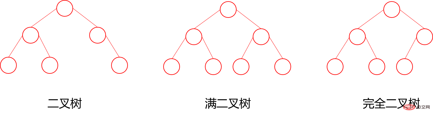
7.4 链式存储的二叉树
创建二叉树:首先需要一个树的类,还需要另一个类用来存放节点,设置节点;将节点放入树中,就形成了二叉树;(节点中需要权值,左子树,右子树,并且都能对他们的值进行设置)。
树的遍历:
-
先序遍历:根节点,左节点,右节点(如果节点有子树,先从左往右遍历子树,再遍历兄弟节点)
先序遍历结果为:A B D H I E J C F K G
-
中序遍历:左节点,根节点,右节点(中序遍历可以看成,二叉树每个节点,垂直方向投影下来(可以理解为每个节点从最左边开始垂直掉到地上),然后从左往右数)
中遍历结果为:H D I B E J A F K C G
-
后序遍历:左节点,右节点,根节点
后序遍历结果:H I D J E B K F G C A
-
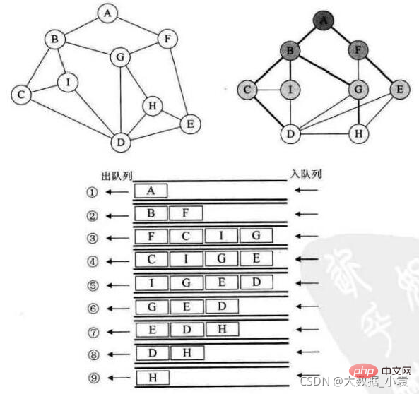
层次遍历:从上往下,从左往右
层次遍历结果:A B C D E F G H I J K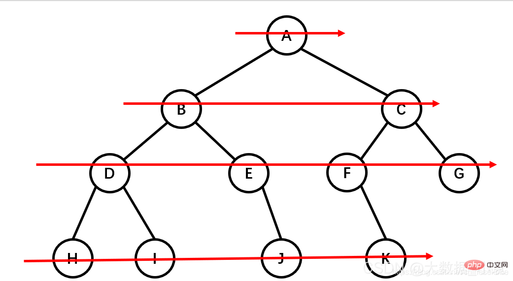
查找节点:先对树进行一次遍历,然后找出要找的那个数;因为有三种排序方法,所以查找节点也分为先序查找,中序查找,后序查找;
删除节点:由于链式存储,不能找到要删的数直接删除,需要找到他的父节点,然后将指向该数设置为null;所以需要一个变量来指向父节点,找到数后,再断开连接。
代码实现:
- 树类
public class BinaryTree {

    TreeNode root;

    //设置根节点
    public void setRoot(TreeNode root) {
        this.root = root;
    }

    //获取根节点
    public TreeNode getRoot() {
        return root;
    }

    //先序遍历
    public void frontShow() {
        if (root != null) {
            root.frontShow();
        }
    }

    //中序遍历
    public void middleShow() {
        if (root != null) {
            root.middleShow();
        }
    }

    //后序遍历
    public void afterShow() {
        if (root != null) {
            root.afterShow();
        }
    }

    //先序查找
    public TreeNode frontSearch(int i) {
        return root.frontSearch(i);
    }

    //删除一个子树
    public void delete(int i) {
        if (root.value == i) {
            root = null;
        } else {
            root.delete(i);
        }
    }}
- 节点类
public class TreeNode {
    //节点的权
    int value;
    //左儿子
    TreeNode leftNode;
    //右儿子
    TreeNode rightNode;

    public TreeNode(int value) {
        this.value = value;
    }

    //设置左儿子
    public void setLeftNode(TreeNode leftNode) {
        this.leftNode = leftNode;
    }

    //设置右儿子
    public void setRightNode(TreeNode rightNode) {
        this.rightNode = rightNode;
    }

    //先序遍历
    public void frontShow() {
        //先遍历当前节点的值
        System.out.print(value + " ");
        //左节点
        if (leftNode != null) {
            leftNode.frontShow(); //递归思想
        }
        //右节点
        if (rightNode != null) {
            rightNode.frontShow();
        }
    }

    //中序遍历
    public void middleShow() {
        //左节点
        if (leftNode != null) {
            leftNode.middleShow(); //递归思想
        }
        //先遍历当前节点的值
        System.out.print(value + " ");
        //右节点
        if (rightNode != null) {
            rightNode.middleShow();
        }
    }

    //后续遍历
    public void afterShow() {
        //左节点
        if (leftNode != null) {
            leftNode.afterShow(); //递归思想
        }
        //右节点
        if (rightNode != null) {
            rightNode.afterShow();
        }
        //先遍历当前节点的值
        System.out.print(value + " ");
    }

    //先序查找
    public TreeNode frontSearch(int i) {
        TreeNode target = null;
        //对比当前节点的值
        if (this.value == i) {
            return this;
            //当前节点不是要查找的节点
        } else {
            //查找左儿子
            if (leftNode != null) {
                //查找的话t赋值给target,查不到target还是null
                target = leftNode.frontSearch(i);
            }
            //如果target不为空,说明在左儿子中已经找到
            if (target != null) {
                return target;
            }
            //如果左儿子没有查到,再查找右儿子
            if (rightNode != null) {
                target = rightNode.frontSearch(i);
            }
        }
        return target;
    }

    //删除一个子树
    public void delete(int i) {
        TreeNode parent = this;
        //判断左儿子
        if (parent.leftNode != null && parent.leftNode.value == i) {
            parent.leftNode = null;
            return;
        }
        //判断右儿子
        if (parent.rightNode != null && parent.rightNode.value == i) {
            parent.rightNode = null;
            return;
        }
        //如果都不是,递归检查并删除左儿子
        parent = leftNode;
        if (parent != null) {
            parent.delete(i);
        }
        //递归检查并删除右儿子
        parent = rightNode;
        if (parent != null) {
            parent.delete(i);
        }

    }}
- 测试类
public class Demo {
    public static void main(String[] args) {
        //创建一棵树
        BinaryTree binaryTree = new BinaryTree();
        //创建一个根节点
        TreeNode root = new TreeNode(1);
        //把根节点赋给树
        binaryTree.setRoot(root);
        //创建左,右节点
        TreeNode rootLeft = new TreeNode(2);
        TreeNode rootRight = new TreeNode(3);
        //把新建的节点设置为根节点的子节点
        root.setLeftNode(rootLeft);
        root.setRightNode(rootRight);
        //为第二层的左节点创建两个子节点
        rootLeft.setLeftNode(new TreeNode(4));
        rootLeft.setRightNode(new TreeNode(5));
        //为第二层的右节点创建两个子节点
        rootRight.setLeftNode(new TreeNode(6));
        rootRight.setRightNode(new TreeNode(7));

        //先序遍历
        binaryTree.frontShow(); //1 2 4 5 3 6 7
        System.out.println();
        //中序遍历
        binaryTree.middleShow(); //4 2 5 1 6 3 7
        System.out.println();
        //后序遍历
        binaryTree.afterShow(); //4 5 2 6 7 3 1
        System.out.println();

        //先序查找
        TreeNode result = binaryTree.frontSearch(5);
        System.out.println(result); //binarytree.TreeNode@1b6d3586

        //删除一个子树
        binaryTree.delete(2);
        binaryTree.frontShow(); //1 3 6 7 ,2和他的子节点被删除了
    }}
7.5 顺序存储的二叉树

概述:顺序存储使用数组的形式实现;由于非完全二叉树会导致数组中出现空缺,有的位置不能填上数字,所以顺序存储二叉树通常情况下只考虑完全二叉树
原理: 顺序存储在数组中是按照第一层第二层一次往下存储的,遍历方式也有先序遍历、中序遍历、后续遍历
性质:
- 第n个元素的左子节点是:2*n+1;
- 第n个元素的右子节点是:2*n+2;
- 第n个元素的父节点是:(n-1)/2
代码实现:
- 树类
public class ArrayBinaryTree {

    int[] data;

    public ArrayBinaryTree(int[] data) {
        this.data = data;
    }

    //重载先序遍历方法,不用每次传参数了,保证每次从头开始
    public void frontShow() {
        frontShow(0);
    }

    //先序遍历
    public void frontShow(int index) {
        if (data == null || data.length == 0) {
            return;
        }
        //先遍历当前节点的内容
        System.out.print(data[index] + " ");
        //处理左子树:2*index+1
        if (2 * index + 1
- 测试类
public class Demo {
    public static void main(String[] args) {
        int[] data = {1,2,3,4,5,6,7};
        ArrayBinaryTree tree = new ArrayBinaryTree(data);
        //先序遍历
        tree.frontShow(); //1 2 4 5 3 6 7
    }}
7.6 线索二叉树(Threaded BinaryTree)
为什么使用线索二叉树?
当用二叉链表作为二叉树的存储结构时,可以很方便的找到某个结点的左右孩子;但一般情况下,无法直接找到该结点在某种遍历序列中的前驱和后继结点
原理:n个结点的二叉链表中含有n+1(2n-(n-1)=n+1个空指针域。利用二叉链表中的空指针域,存放指向结点在某种遍历次序下的前驱和后继结点的指针。
例如:某个结点的左孩子为空,则将空的左孩子指针域改为指向其前驱;如果某个结点的右孩子为空,则将空的右孩子指针域改为指向其后继(这种附加的指针称为"线索")
代码实现:
- 树类
public class ThreadedBinaryTree {

    ThreadedNode root;
    //用于临时存储前驱节点
    ThreadedNode pre = null;

    //设置根节点
    public void setRoot(ThreadedNode root) {
        this.root = root;
    }

    //中序线索化二叉树
    public void threadNodes() {
        threadNodes(root);
    }

    public void threadNodes(ThreadedNode node) {
        //当前节点如果为null,直接返回
        if (node == null) {
            return;
        }
        //处理左子树
        threadNodes(node.leftNode);

        //处理前驱节点
        if (node.leftNode == null) {
            //让当前节点的左指针指向前驱节点
            node.leftNode = pre;
            //改变当前节点左指针类型
            node.leftType = 1;
        }
        //处理前驱的右指针,如果前驱节点的右指针是null(没有右子树)
        if (pre != null && pre.rightNode == null) {
            //让前驱节点的右指针指向当前节点
            pre.rightNode = node;
            //改变前驱节点的右指针类型
            pre.rightType = 1;
        }

        //每处理一个节点,当前节点是下一个节点的前驱节点
        pre = node;

        //处理右子树
        threadNodes(node.rightNode);
    }

    //遍历线索二叉树
    public void threadIterate() {
        //用于临时存储当前遍历节点
        ThreadedNode node = root;
        while (node != null) {
            //循环找到最开始的节点
            while (node.leftType == 0) {
                node = node.leftNode;
            }
            //打印当前节点的值
            System.out.print(node.value + " ");
            //如果当前节点的右指针指向的是后继节点,可能后继节点还有后继节点
            while (node.rightType == 1) {
                node = node.rightNode;
                System.out.print(node.value + " ");
            }
            //替换遍历的节点
            node = node.rightNode;

        }
    }

    //获取根节点
    public ThreadedNode getRoot() {
        return root;
    }

    //先序遍历
    public void frontShow() {
        if (root != null) {
            root.frontShow();
        }
    }

    //中序遍历
    public void middleShow() {
        if (root != null) {
            root.middleShow();
        }
    }

    //后序遍历
    public void afterShow() {
        if (root != null) {
            root.afterShow();
        }
    }

    //先序查找
    public ThreadedNode frontSearch(int i) {
        return root.frontSearch(i);
    }

    //删除一个子树
    public void delete(int i) {
        if (root.value == i) {
            root = null;
        } else {
            root.delete(i);
        }
    }}
- 节点类
public class ThreadedNode {
    //节点的权
    int value;
    //左儿子
    ThreadedNode leftNode;
    //右儿子
    ThreadedNode rightNode;
    //标识指针类型,1表示指向上一个节点,0
    int leftType;
    int rightType;

    public ThreadedNode(int value) {
        this.value = value;
    }

    //设置左儿子
    public void setLeftNode(ThreadedNode leftNode) {
        this.leftNode = leftNode;
    }

    //设置右儿子
    public void setRightNode(ThreadedNode rightNode) {
        this.rightNode = rightNode;
    }

    //先序遍历
    public void frontShow() {
        //先遍历当前节点的值
        System.out.print(value + " ");
        //左节点
        if (leftNode != null) {
            leftNode.frontShow(); //递归思想
        }
        //右节点
        if (rightNode != null) {
            rightNode.frontShow();
        }
    }

    //中序遍历
    public void middleShow() {
        //左节点
        if (leftNode != null) {
            leftNode.middleShow(); //递归思想
        }
        //先遍历当前节点的值
        System.out.print(value + " ");
        //右节点
        if (rightNode != null) {
            rightNode.middleShow();
        }
    }

    //后续遍历
    public void afterShow() {
        //左节点
        if (leftNode != null) {
            leftNode.afterShow(); //递归思想
        }
        //右节点
        if (rightNode != null) {
            rightNode.afterShow();
        }
        //先遍历当前节点的值
        System.out.print(value + " ");
    }

    //先序查找
    public ThreadedNode frontSearch(int i) {
        ThreadedNode target = null;
        //对比当前节点的值
        if (this.value == i) {
            return this;
            //当前节点不是要查找的节点
        } else {
            //查找左儿子
            if (leftNode != null) {
                //查找的话t赋值给target,查不到target还是null
                target = leftNode.frontSearch(i);
            }
            //如果target不为空,说明在左儿子中已经找到
            if (target != null) {
                return target;
            }
            //如果左儿子没有查到,再查找右儿子
            if (rightNode != null) {
                target = rightNode.frontSearch(i);
            }
        }
        return target;
    }

    //删除一个子树
    public void delete(int i) {
        ThreadedNode parent = this;
        //判断左儿子
        if (parent.leftNode != null && parent.leftNode.value == i) {
            parent.leftNode = null;
            return;
        }
        //判断右儿子
        if (parent.rightNode != null && parent.rightNode.value == i) {
            parent.rightNode = null;
            return;
        }
        //如果都不是,递归检查并删除左儿子
        parent = leftNode;
        if (parent != null) {
            parent.delete(i);
        }
        //递归检查并删除右儿子
        parent = rightNode;
        if (parent != null) {
            parent.delete(i);
        }

    }}
- 测试类
public class Demo {
    public static void main(String[] args) {
        //创建一棵树
        ThreadedBinaryTree binaryTree = new ThreadedBinaryTree();
        //创建一个根节点
        ThreadedNode root = new ThreadedNode(1);
        //把根节点赋给树
        binaryTree.setRoot(root);
        //创建左,右节点
        ThreadedNode rootLeft = new ThreadedNode(2);
        ThreadedNode rootRight = new ThreadedNode(3);
        //把新建的节点设置为根节点的子节点
        root.setLeftNode(rootLeft);
        root.setRightNode(rootRight);
        //为第二层的左节点创建两个子节点
        rootLeft.setLeftNode(new ThreadedNode(4));
        ThreadedNode fiveNode = new ThreadedNode(5);
        rootLeft.setRightNode(fiveNode);
        //为第二层的右节点创建两个子节点
        rootRight.setLeftNode(new ThreadedNode(6));
        rootRight.setRightNode(new ThreadedNode(7));

        //中序遍历
        binaryTree.middleShow(); //4 2 5 1 6 3 7
        System.out.println();
        //中序线索化二叉树
        binaryTree.threadNodes();//        //获取5的后继节点//        ThreadedNode afterFive = fiveNode.rightNode;//        System.out.println(afterFive.value); //1
        binaryTree.threadIterate(); //4 2 5 1 6 3 7
    }}
7.7 二叉排序树(Binary Sort Tree)
无序序列: 二叉排序树图解:
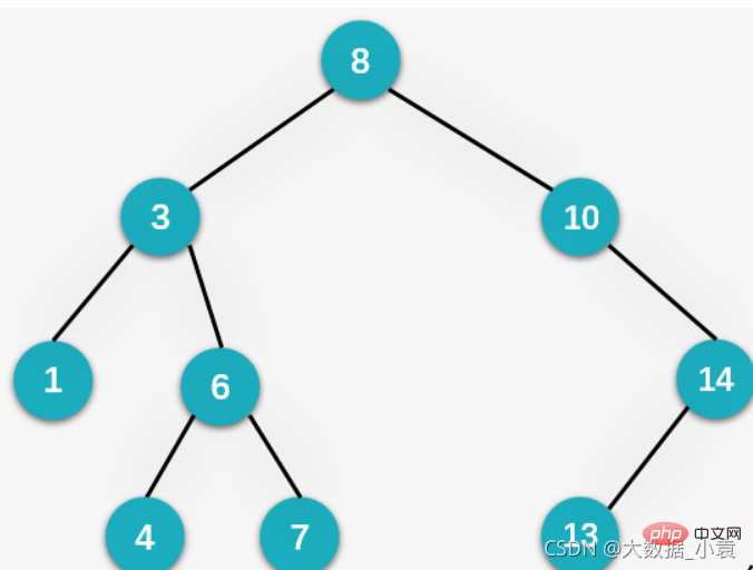
概述:二叉排序树(Binary Sort Tree)也叫二叉查找树或者是一颗空树,对于二叉树中的任何一个非叶子节点,要求左子节点比当前节点值小,右子节点比当前节点值大
特点:
- 查找性能与插入删除性能都适中还不错
- 中序遍历的结果刚好是从大到小
创建二叉排序树原理:其实就是不断地插入节点,然后进行比较。
删除节点
- 删除叶子节点,只需要找到父节点,将父节点与他的连接断开即可
- 删除有一个子节点的就需要将他的子节点换到他现在的位置
- 删除有两个子节点的节点,需要使用他的前驱节点或者后继节点进行替换,就是左子树最右下方的数(最大的那个)或右子树最左边的树(最小的数);即离节点值最接近的值;(还要注解要去判断这个值有没有右节点,有就要将右节点移上来)
代码实现:
- 树类
public class BinarySortTree {
    Node root;

    //添加节点
    public void add(Node node) {
        //如果是一颗空树
        if (root == null) {
            root = node;
        } else {
            root.add(node);
        }
    }

    //中序遍历
    public void middleShow() {
        if (root != null) {
            root.middleShow(root);
        }
    }

    //查找节点
    public Node search(int value) {
        if (root == null) {
            return null;
        }
        return root.search(value);
    }

    //查找父节点
    public Node searchParent(int value) {
        if (root == null) {
            return null;
        }
        return root.searchParent(value);
    }

    //删除节点
    public void delete(int value) {
        if (root == null) {
            return;
        } else {
            //找到这个节点
            Node target = search(value);
            //如果没有这个节点
            if (target == null) {
                return;
            }
            //找到他的父节点
            Node parent = searchParent(value);
            //要删除的节点是叶子节点
            if (target.left == null && target.left == null) {
                //要删除的节点是父节点的左子节点
                if (parent.left.value == value) {
                    parent.left = null;
                }
                //要删除的节点是父节点的右子节点
                else {
                    parent.right = null;
                }
            }
            //要删除的节点有两个子节点的情况
            else if (target.left != null && target.right != null) {
                //删除右子树中值最小的节点,并且获取到值
                int min = deletMin(target.right);
                //替换目标节点中的值
                target.value = min;
            }
            //要删除的节点有一个左子节点或右子节点
            else {
                //有左子节点
                if (target.left != null) {
                    //要删除的节点是父节点的左子节点
                    if (parent.left.value == value) {
                        parent.left = target.left;
                    }
                    //要删除的节点是父节点的右子节点
                    else {
                        parent.right = target.left;
                    }

                }
                //有右子节点
                else {
                    //要删除的节点是父节点的左子节点
                    if (parent.left.value == value) {
                        parent.left = target.right;
                    }
                    //要删除的节点是父节点的右子节点
                    else {
                        parent.right = target.right;
                    }
                }
            }
        }
    }

    //删除一棵树中最小的节点
    private int deletMin(Node node) {
        Node target = node;
        //递归向左找最小值
        while (target.left != null) {
            target = target.left;
        }
        //删除最小的节点
        delete(target.value);
        return target.value;
    }}
- 节点类
public class Node {
    int value;
    Node left;
    Node right;

    public Node(int value) {
        this.value = value;
    }

    //向子树中添加节点
    public void add(Node node) {
        if (node == null) {
            return;
        }
        /*判断传入的节点的值比当前紫薯的根节点的值大还是小*/
        //添加的节点比当前节点更小(传给左节点)
        if (node.value  value && this.left != null) {
                return this.left.searchParent(value);
            } else if (this.value
- 测试类
public class Demo {
    public static void main(String[] args) {
        int[] arr = {8, 3, 10, 1, 6, 14, 4, 7, 13};
        //创建一颗二叉排序树
        BinarySortTree bst = new BinarySortTree();
        //循环添加/*        for(int i=0;i<h2>7.8 平衡二叉树( Balanced Binary Tree)</h2><h3>为什么使用平衡二叉树?</h3><p>平衡二叉树(Balanced Binary Tree)又被称为AVL树,且具有以下性质:它是一棵空树或它的左右两个子树的高度差的绝对值不超过1,并且左右两个子树都是一棵平衡二叉树。这个方案很好的解决了二叉查找树退化成链表的问题,把插入,查找,删除的时间复杂度最好情况和最坏情况都维持在<code>O(logN)</code>。但是频繁旋转会使插入和删除牺牲掉<code>O(logN)</code>左右的时间,不过相对二叉查找树来说,时间上稳定了很多。</p><p>二叉排序树插入 {1,2,3,4,5,6} 这种数据结果如下图所示:<br><img src="https://img.php.cn/upload/article/000/000/067/3ecfcc25f4c8b7a56d063b2b27bace0c-23.png" alt="Detailed graphic explanation of Java data structures and algorithms"><br> 平衡二叉树插入 {1,2,3,4,5,6} 这种数据结果如下图所示:<br><img src="https://img.php.cn/upload/article/000/000/067/3ecfcc25f4c8b7a56d063b2b27bace0c-24.png" alt="Detailed graphic explanation of Java data structures and algorithms"></p><h3>如何判断平衡二叉树?</h3>
- 1、是二叉排序树
- 2、任何一个节点的左子树或者右子树都是平衡二叉树(左右高度差小于等于 1)
(1)下图不是平衡二叉树,因为它不是二叉排序树违反第 1 条件
(2)下图不是平衡二叉树,因为有节点子树高度差大于 1 违法第 2 条件(5的左子树为0,右子树为2)
(3)下图是平衡二叉树,因为符合 1、2 条件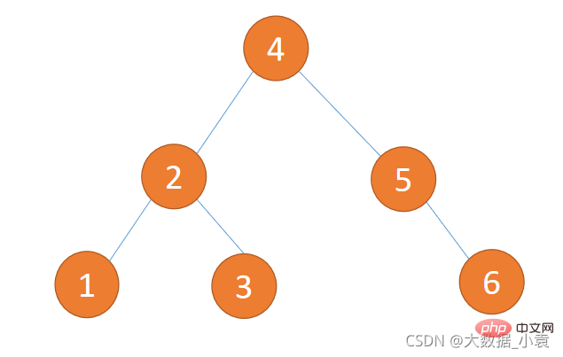
相关概念
平衡因子 BF
- Definition: The height difference between the left subtree and the right subtree
- Calculation:
The height of the left subtree - the value of the height of the right subtree - Alias: Abbreviated as BF (Balance Factor)
- Generally speaking, if the absolute value of BF is greater than 1, the balanced tree binary tree will be unbalanced and needs to be rotated to correct
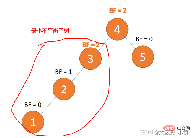
Minimum unbalanced subtree
#The node closest to the inserted node and with an absolute value of BF greater than 1 is the subtree of the root node.
Rotation correction only needs to correct the minimum unbalanced subtree
An example is shown in the figure below:
Rotation method
2 rotation methods:
Left rotation:
- The old root node is The left subtree of the new root node
- The left subtree of the new root node (if it exists) is the right subtree of the old root node
Right rotation:
- The old root node is the right subtree of the new root node
- The right subtree of the new root node (if it exists) is the left subtree of the old root node
4 types of rotation correction:
- Left-left type: insert the left subtree of the left child, right rotation
- Right-right type: insert the right subtree of the right child , Left-handed type
- Left-left type: Insert the right subtree of the left child, first rotate left, then rotate right
- Right-left type: Insert the left subtree of the right child, first rotate right, then rotate left
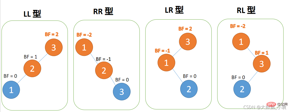
Left-left type:
When the third node (1) is inserted, BF(3) = 2, BF(2) = 1, right-handed, root node rotates clockwise
Right-right type:
The third node (3) When inserting, BF(1)=-2 BF(2)=-1, RR type unbalanced, left-handed, root node rotates counterclockwise
left-right type :
When the third node (3) is inserted, BF(3)=2 BF(1)=-1 LR type imbalance, first left-handed and then right-handed
Right-left type:
When the third node (1) is inserted, BF(1)=-2 BF(3)=1 RL type imbalance, first right-hand rotation and then left-hand rotation
Example
(1), Insert 3, 2, and 1 in sequence. When inserting the third point 1, BF(3)=2 BF(2)=1, LL type imbalance, for the minimum unbalanced tree {3,2,1} Perform right rotation
- The old root node (node 3) is the right subtree of the new root node (node 2)
- The right subtree of the new root node (node 2) (here No right subtree) is the left subtree of the old root node

(2) Insert 4 and 5 in sequence. When inserting 5 pointsBF(3) = - 2 BF(4)=-1, RR type imbalance, perform left rotation on the minimum unbalanced tree {3,4,5}
- The old root node (node 3) is the new root node The left subtree of (node 4)
- The left subtree of the new root node (node 4) (there is no left subtree here) is the right subtree of the old root node

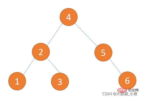
(3) When inserting 4 and 5 into 5 points, BF(2)=-2 BF(4)=-1, RR type imbalance is the minimum imbalance tree {1,2 ,4} Perform left rotation
- The old root node (node 2) is the left subtree of the new root node (node 4)

- The new root node (node 4) The left subtree (node 3) is the right subtree of the old root node

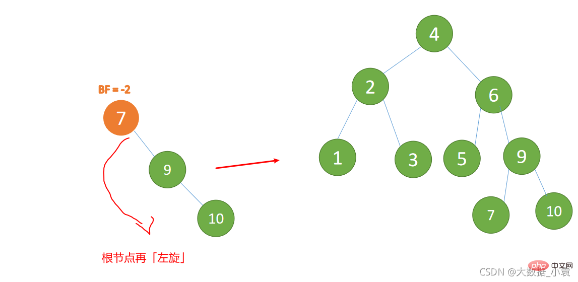
(4) When inserting node 7BF(5)=- 2, BF(6)=-1, RR type imbalance, left-handed rotation of the minimum imbalance tree
- 旧根节点(节点 5)为新根节点(节点 6)的左子树
- 新根节点的左子树(这里没有)为旧根节点的右子树
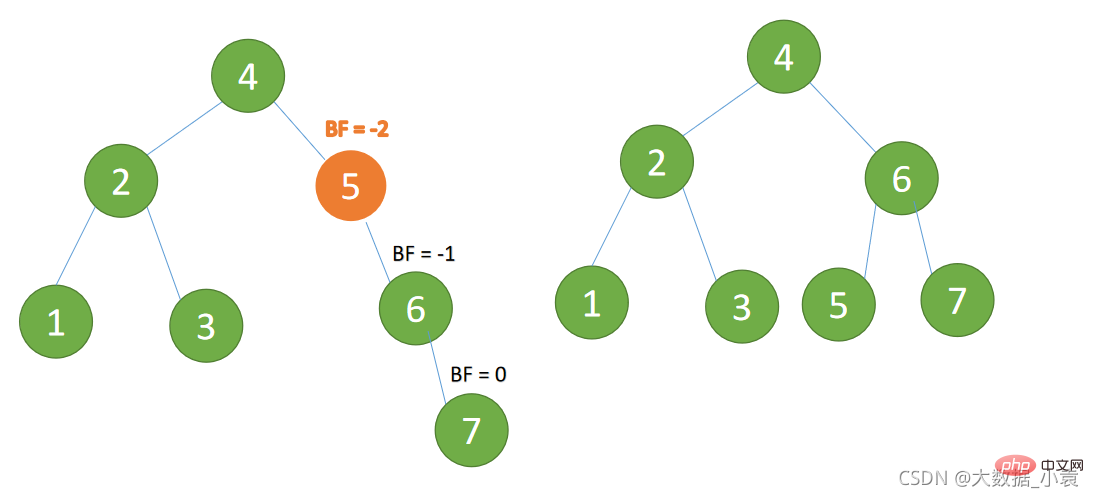
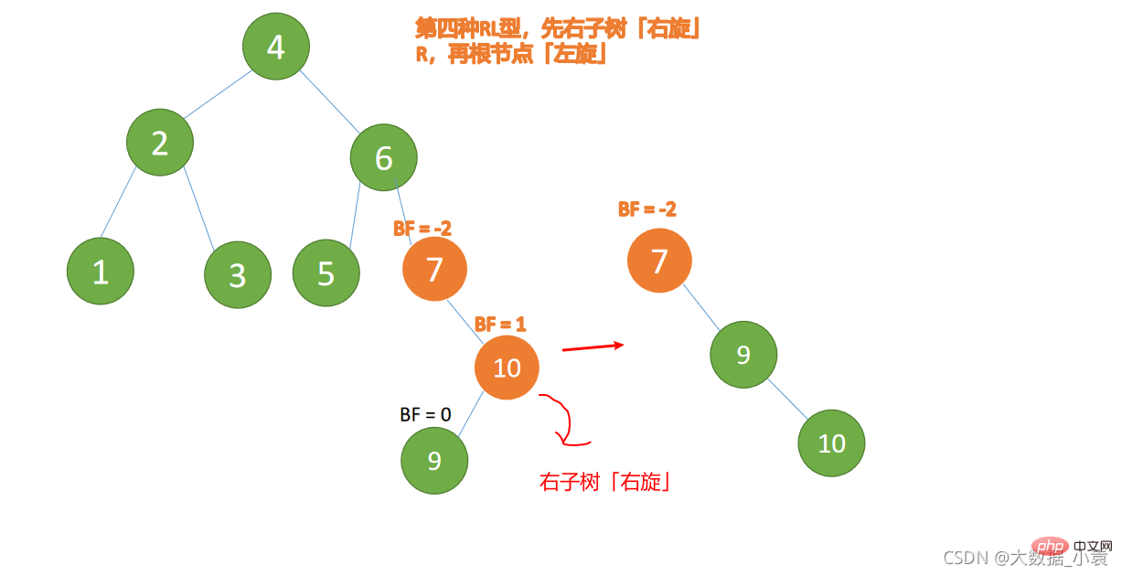
(5)依次插入 10 ,9 。插入 9 点的时候 BF(10) = 1,BF(7) = -2,RL 型失衡,对先右旋再左旋,右子树先右旋
- 旧根节点(节点 10)为新根节点(节点 9)的右子树
- 新根节点(节点 9)的右子树(这里没有右子树)为旧根节点的左子树
最小不平衡子树再左旋: - 旧根节点(节点 7)为新根节点(节点 9)的左子树
- 新根节点(节点 9)的左子树(这里没有左子树)为旧根节点的右子树
代码实现
- 节点类
public class Node {
    int value;
    Node left;
    Node right;

    public Node(int value) {
        this.value = value;
    }

    //获取当前节点高度
    public int height() {
        return Math.max(left == null ? 0 : left.height(), right == null ? 0 : right.height()) + 1;
    }

    //获取左子树高度
    public int leftHeight() {
        if (left == null) {
            return 0;
        }
        return left.height();
    }

    //获取右子树高度
    public int rightHeight() {
        if (right == null) {
            return 0;
        }
        return right.height();
    }


    //向子树中添加节点
    public void add(Node node) {
        if (node == null) {
            return;
        }
        /*判断传入的节点的值比当前紫薯的根节点的值大还是小*/
        //添加的节点比当前节点更小(传给左节点)
        if (node.value = 2) {
            //双旋转,当左子树左边高度小于左子树右边高度时
            if (left != null && left.leftHeight()  value && this.left != null) {
                return this.left.searchParent(value);
            } else if (this.value
- 测试类
public class Demo {
    public static void main(String[] args) {
        int[] arr = {1,2,3,4,5,6};
        //创建一颗二叉排序树
        BinarySortTree bst = new BinarySortTree();
        //循环添加
        for (int i : arr) {
            bst.add(new Node(i));
        }
        //查看高度
        System.out.println(bst.root.height()); //3
        //查看节点值
        System.out.println(bst.root.value); //根节点为4
        System.out.println(bst.root.left.value); //左子节点为2
        System.out.println(bst.root.right.value); //右子节点为5
    }}
第8章 赫夫曼树
8.1 赫夫曼树概述
HuffmanTree因为翻译不同所以有其他的名字:赫夫曼树、霍夫曼树、哈夫曼树
赫夫曼树又称最优二叉树,是一种带权路径长度最短的二叉树。所谓树的带权路径长度,就是树中所有的叶结点的权值乘上其到根结点的路径长度(若根结点为0层,叶结点到根结点的路径长度为叶结点的层数)。树的路径长度是从树根到每一结点的路径长度之和,记为WPL=(W1L1+W2L2+W3L3+…+WnLn),N个权值Wi(i=1,2,…n)构成一棵有N个叶结点的二叉树,相应的叶结点的路径长度为Li(i=1,2,…n)。可以证明赫夫曼树的WPL是最小的。
8.2 赫夫曼树定义
路径: 路径是指从一个节点到另一个节点的分支序列。
路径长度: 指从一个节点到另一个结点所经过的分支数目。 如下图:从根节点到a的分支数目为2
树的路径长度: 树中所有结点的路径长度之和为树的路径长度PL。 如下图:PL为10
节点的权: 给树的每个结点赋予一个具有某种实际意义的实数,我们称该实数为这个结点的权。如下图:7、5、2、4
带权路径长度: 从树根到某一结点的路径长度与该节点的权的乘积,叫做该结点的带权路径长度。如下图:A的带权路径长度为2*7=14
树的带权路径长度(WPL): 树的带权路径长度为树中所有叶子节点的带权路径长度之和
最优二叉树:权值最大的节点离跟节点越近的二叉树,所得WPL值最小,就是最优二叉树。如下图:(b)
- (a)
WPL=9*2+4*2+5*2+2*2=40 - (b)
WPL=9*1+5*2+4*3+2*3=37 - (c)
WPL=4*1+2*2+5*3+9*3=50
8.3 构造赫夫曼树步骤
对于数组{5,29,7,8,14,23,3,11},我们把它构造成赫夫曼树
第一步:使用数组中所有元素创建若干个二叉树,这些值作为节点的权值(只有一个节点)。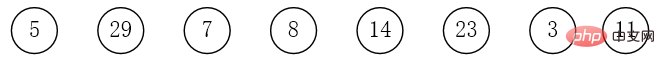
第二步:将这些节点按照权值的大小进行排序。
第三步:取出权值最小的两个节点,并创建一个新的节点作为这两个节点的父节点,这个父节点的权值为两个子节点的权值之和。将这两个节点分别赋给父节点的左右节点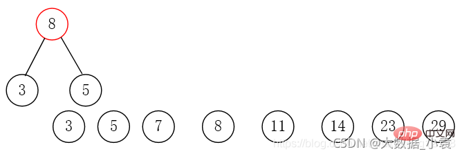
第四步:删除这两个节点,将父节点添加进集合里
第五步:重复第二步到第四步,直到集合中只剩一个元素,结束循环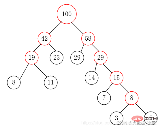
8.4 代码实现
- 节点类
//接口实现排序功能public class Node implements Comparable<node> {
    int value;
    Node left;
    Node right;

    public Node(int value) {
        this.value = value;
    }

    @Override
    public int compareTo(Node o) {
        return -(this.value - o.value); //集合倒叙,从大到小
    }

    @Override
    public String toString() {
        return "Node value=" + value ;
    }}</node>
- 测试类
import java.util.ArrayList;import java.util.Collections;import java.util.List;public class Demo {
    public static void main(String[] args) {
        int[] arr = {5, 29, 7, 8, 14, 23, 3, 11};
        Node node = createHuffmanTree(arr);
        System.out.println(node); //Node value=100
    }

    //创建赫夫曼树
    public static Node createHuffmanTree(int[] arr) {
        //使用数组中所有元素创建若干个二叉树(只有一个节点)
        List<node> nodes = new ArrayList();
        for (int value : arr) {
            nodes.add(new Node(value));
        }

        //循环处理
        while (nodes.size() > 1) {
            //排序
            Collections.sort(nodes);
            //取出最小的两个二叉树(集合为倒叙,从大到小)
            Node left = nodes.get(nodes.size() - 1); //权值最小
            Node right = nodes.get(nodes.size() - 2); //权值次小
            //创建一个新的二叉树
            Node parent = new Node(left.value + right.value);
            //删除原来的两个节点
            nodes.remove(left);
            nodes.remove(right);
            //新的二叉树放入原来的二叉树集合中
            nodes.add(parent);
            //打印结果
            System.out.println(nodes);
        }
        return nodes.get(0);
    }}</node>
- 循环次数结果
[Node value=29, Node value=23, Node value=14, Node value=11, Node value=8, Node value=7, Node value=8][Node value=29, Node value=23, Node value=14, Node value=11, Node value=8, Node value=15][Node value=29, Node value=23, Node value=15, Node value=14, Node value=19][Node value=29, Node value=23, Node value=19, Node value=29][Node value=29, Node value=29, Node value=42][Node value=42, Node value=58][Node value=100]Node value=100Process finished with exit code 0
第9章 多路查找树(2-3树、2-3-4树、B树、B+树)
9.1 为什么使用多路查找树
二叉树存在的问题
二叉树需要加载到内存的,如果二叉树的节点少,没有什么问题,但是如果二叉树的节点很多(比如1亿), 就存在如下问题:
问题1:在构建二叉树时,需要多次进行I/O操作(海量数据存在数据库或文件中),节点海量,构建二叉树时,
速度有影响.问题2:节点海量,也会造成二叉树的
高度很大,会降低操作速度.
解决上述问题 —> 多叉树
多路查找树
- 1、在二叉树中,每个节点有数据项,最多有两个子节点。如果允许每个节点可以有
更多的数据项和更多的子节点,就是多叉树(multiway tree) - 2、后面我们讲解的"2-3树","2-3-4树"就是多叉树,多叉树通过
重新组织节点,减少树的高度,能对二叉树进行优化。 - 3、举例说明(下面2-3树就是一颗多叉树)

9.2 2-3树
2-3树定义
- 所有叶子节点都要在同一层
- 二节点要么有两个子节点,要么没有节点
- 三节点要么没有节点,要么有三个子节点
- 不能出现节点不满的情况

2-3树插入的操作
插入原理:
对于2-3树的插入来说,与平衡二叉树相同,插入操作一定是发生在叶子节点上,并且节点的插入和删除都有可能导致不平衡的情况发生,在插入和删除节点时也是需要动态维持平衡的,但维持平衡的策略和AVL树是不一样的。
AVL树向下添加节点之后通过旋转来恢复平衡,而2-3树是通过节点向上分裂来维持平衡的,也就是说2-3树插入元素的过程中层级是向上增加的,因此不会导致叶子节点不在同一层级的现象发生,也就不需要旋转了。
三种插入情况:
1)对于空树,插入一个2节点即可;
2)插入节点到一个2节点的叶子上。由于本身就只有一个元素,所以只需要将其升级为3节点即可(如:插入3)。

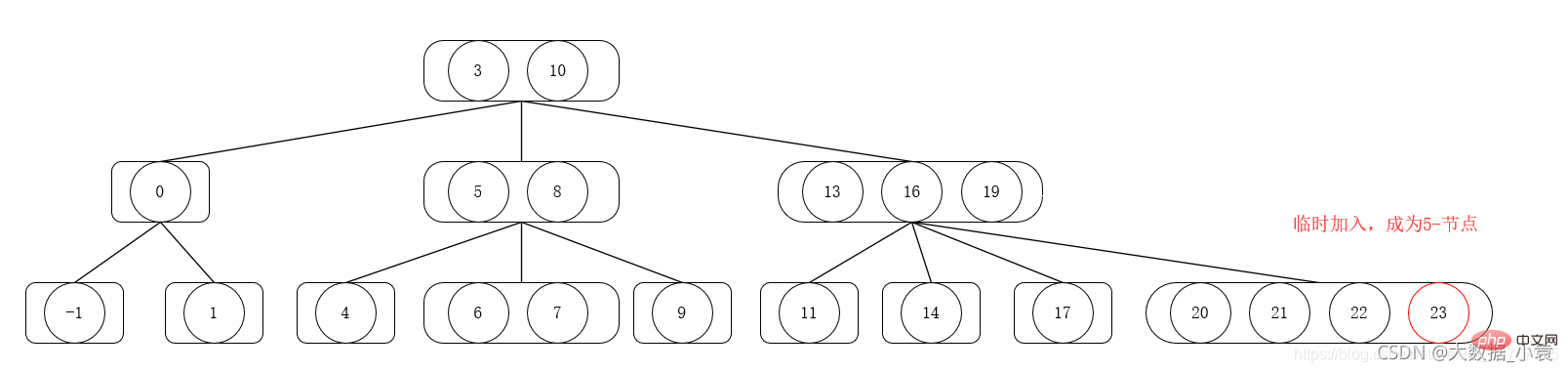
3)插入节点到一个3节点的叶子上。因为3节点本身最大容量,因此需要拆分,且将树中两元素或者插入元素的三者中选择其一向上移动一层。
分为三种情况:
- 升级父节点(插入5)

- 升级根节点(插入11)

- 增加树高度(插入2,从下往上拆)

2-3树删除的操作
删除原理:2-3树的删除也分为三种情况,与插入相反。
三种删除情况:
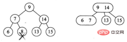
1) The deleted element is located on a leaf node of 3 nodes. Deleting it directly will not affect the tree structure (such as deleting 9) 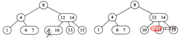
2) The deleted element is located on a 2 node , delete it directly and destroy the tree structure 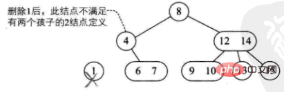
It is divided into four situations:
The parents of this node are also 2 nodes, and have a 3-node Right child (eg: delete 1)

The parent of this node is node 2, and its right child is also node 2 (eg: delete 4)
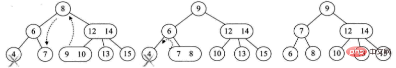
The parents of this node are 3 nodes (for example: delete 10)
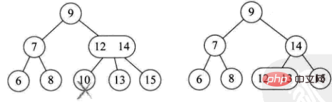
The current tree is a full tree Binary tree, reduce the tree height (for example: delete 8)
3) The deleted element is located at a non-leaf branch node. At this time, the predecessor or subsequent elements of this element are obtained by traversing the tree in order, and the filling
has two situations:
- The branch node is 2 nodes (for example: delete 4)
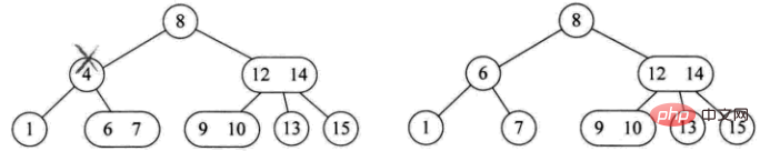
- The branch node is 3 nodes (for example: delete 12)


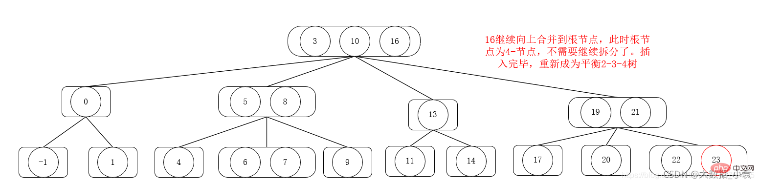

The data structure of the B-tree is prepared for data interaction between internal and external memory. When the data to be processed is large, it cannot be loaded into memory all at once. At this time, the B-tree is adjusted so that the order of the B-tree matches the page size stored in the hard disk. For example, a B-tree has an order of 1001 (that is, 1 node contains 1000 keywords) and a height of 2 (starting from 0). It can store more than 1 billion keywords (1001x1001x1000 1001x1000 1000). As long as the root node If it is persisted in memory, then searching for a certain keyword in this tree requires at most two hard disk reads.
For an m-order B-tree with n keywords, Calculation of worst-case search times
There must be at least 1 node in the first level and at least 2 nodes in the second level. Since every node except the root node Each branch node has at least ⌈m/2⌉ subtrees, then the third level has at least 2x⌈m/2⌉ nodes. . . In this way, the k 1th layer has at least 2x(⌈m/2⌉)^(k-1). In fact, the nodes in the k 1th layer are leaf nodes. If the m-order B-tree has n keywords, then when you find the leaf node, it actually means that the unsuccessful node is n 1, so
n 1>=2x(⌈m/2⌉)^(k -1), that is, 
When searching on a B-tree containing n keywords, the number of nodes involved in the path from the root node to the keyword node is not too many
9.5 B-tree
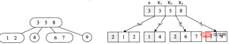
B-tree can be said to be an upgraded version of B-tree. Compared with B-tree, B-tree makes full use of the node space and makes the query speed more stable. The speed is completely close to binary search. Most file systems and data use B-trees to implement index structures.
We need to traverse the B-tree in the figure below. Assume that each node belongs to a different page on the hard disk. We traverse all the elements in order, page 2-page 1-page 3-page 1-page 4. - Page 1 - Page 5, page 1 has been traversed 3 times, and every time we traverse a node, we will traverse the elements in the node once. 
B The tree is the file system. A deformed tree of the B-tree. In the B-tree, each element appears only once in the tree. In the B-tree, the elements that appear in the branch node will be regarded as their in-order position in the branch node. Listed again in successors (leaf nodes). In addition, each leaf node will save a pointer to the following leaf node.
The picture below is a B-tree. Gray keywords appear at the root node and are listed again in the leaf nodes. 
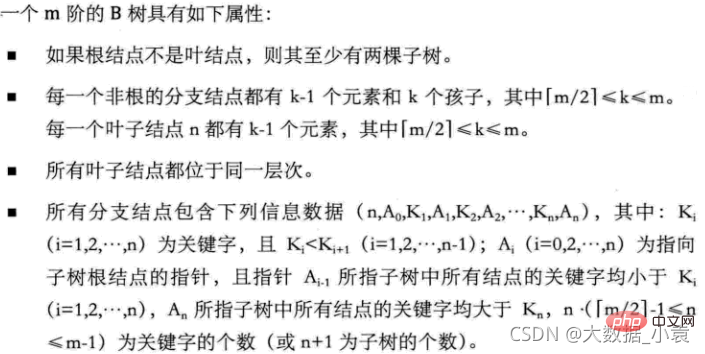
A B-tree of order m and order m The difference between the B-tree is :
- There are n sub-trees whose non-leaf nodes contain n keywords (n-1 keywords in the B-tree), but each Keywords do not save data, but are only used to save indexes of the same keywords in leaf nodes. All data is stored in leaf nodes. (Here, for the relationship between m subtrees and n keywords of non-leaf nodes, the index structure of mysql seems to be m=n 1, not the above m=n)
- All non-leaf nodes Node elements all exist in child nodes at the same time, and it is the largest (or smallest) element among child node elements.
- All leaf nodes contain information about all keywords and pointer data to the specific disk records pointed to by these keywords, and each leaf node has a pointer to the next adjacent leaf node. Forming a linked list
9.6 Summary
The non-leaf nodes of the B-tree will store keywords and their corresponding data addresses, and the non-leaf nodes of the B-tree only store Keyword index does not store specific data addresses, so a node of the B-tree can store more index elements than the B-tree, and the more keywords need to be searched when read into the memory at one time, the height of the B-tree Smaller, the relative number of IO reads and writes is reduced.
The query efficiency of the B-tree is not stable. In the best case, it only queries once (the root node). In the worst case, the leaf nodes are found. However, the B-tree does not The data address is stored, but only the index of the key in the leaf node. All queries must find leaf nodes to be considered hits, and the query efficiency is relatively stable. This is very helpful for optimizing SQL statements.
All leaf nodes of the B tree form an ordered linked list, and the entire tree can be traversed only by traversing the leaf nodes. It is convenient for range query of data, but B-tree does not support such operation or is too inefficient.
Most of the index tables in modern databases and file systems are implemented using B-trees, but not all
Chapter 10 Figure Structure
10.1 The basic concept of graph
Graph (Graph) is a complex nonlinear structure. In the graph structure, each element can have zero or multiple predecessors, and can have zero or more successors, that is, the relationship between elements is arbitrary.
Commonly used terms:
| Term | Meaning |
|---|---|
| Someone in the graph Nodes | |
| Connections between vertices | |
| are connected by the same Vertices connected by edges | |
| Number of adjacent vertices of a vertex | |
| A route from one vertex to another without passing through the vertex repeatedly | |
| The starting point and the end point are both the same vertex | |
| All edges in the graph have no direction | |
| All edges in the graph The edges have directions | |
| The edges in the graph have no weight value | |
| The edges in the graph have a certain weight value |


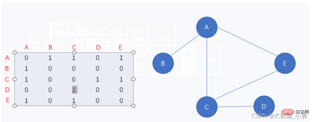 图中的 0 表示该顶点无法通向另一个顶点,相反 1 就表示该顶点能通向另一个顶点

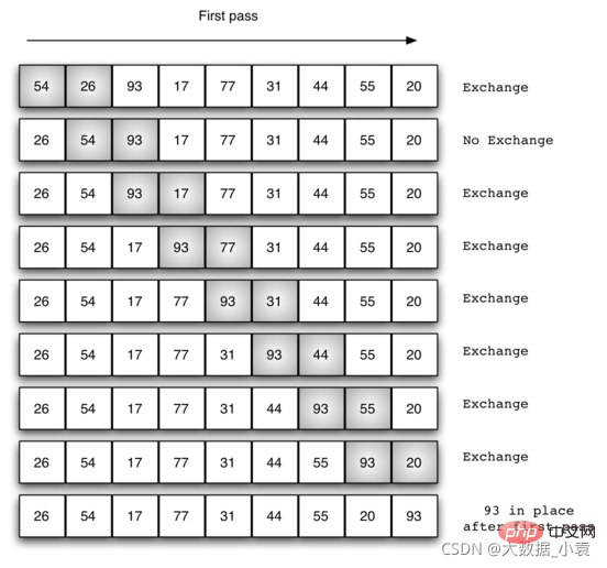 那么我们需要进行n-1次冒泡过程,每次对应的比较次数如下图所示:
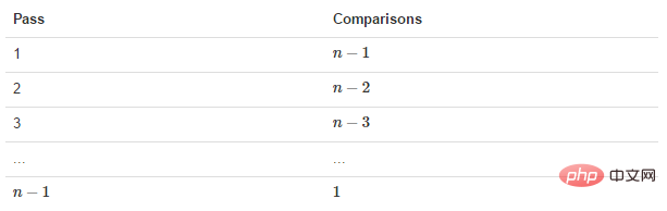


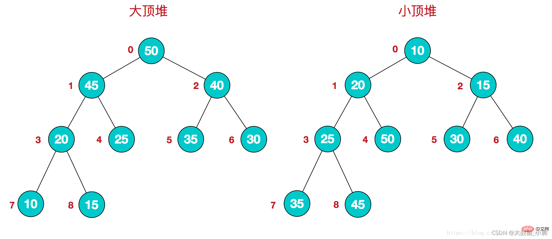 同时,我们对堆中的结点按层进行编号,将这种逻辑结构映射到数组中就是下面这个样子
 该数组从逻辑上讲就是一个堆结构,我们用简单的公式来描述一下堆的定义就是:
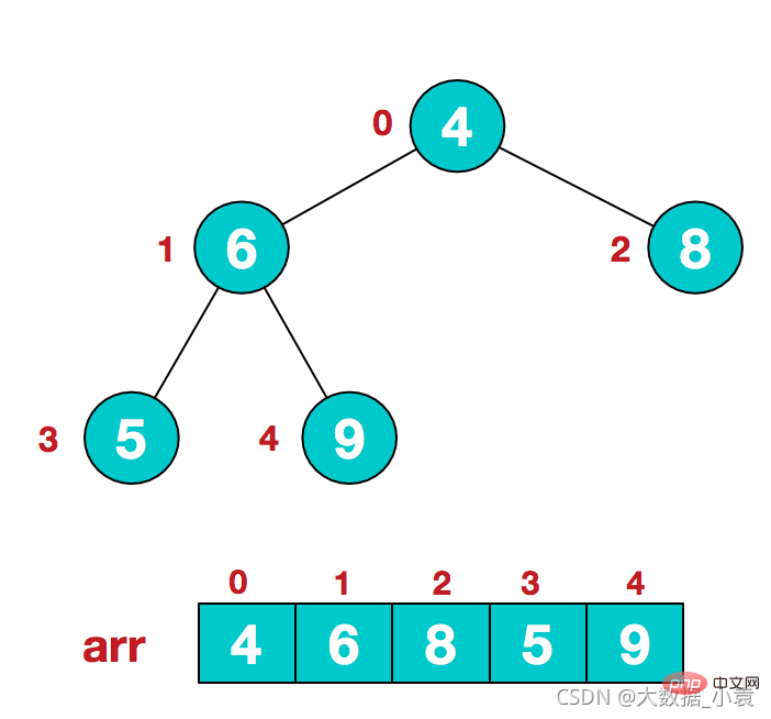
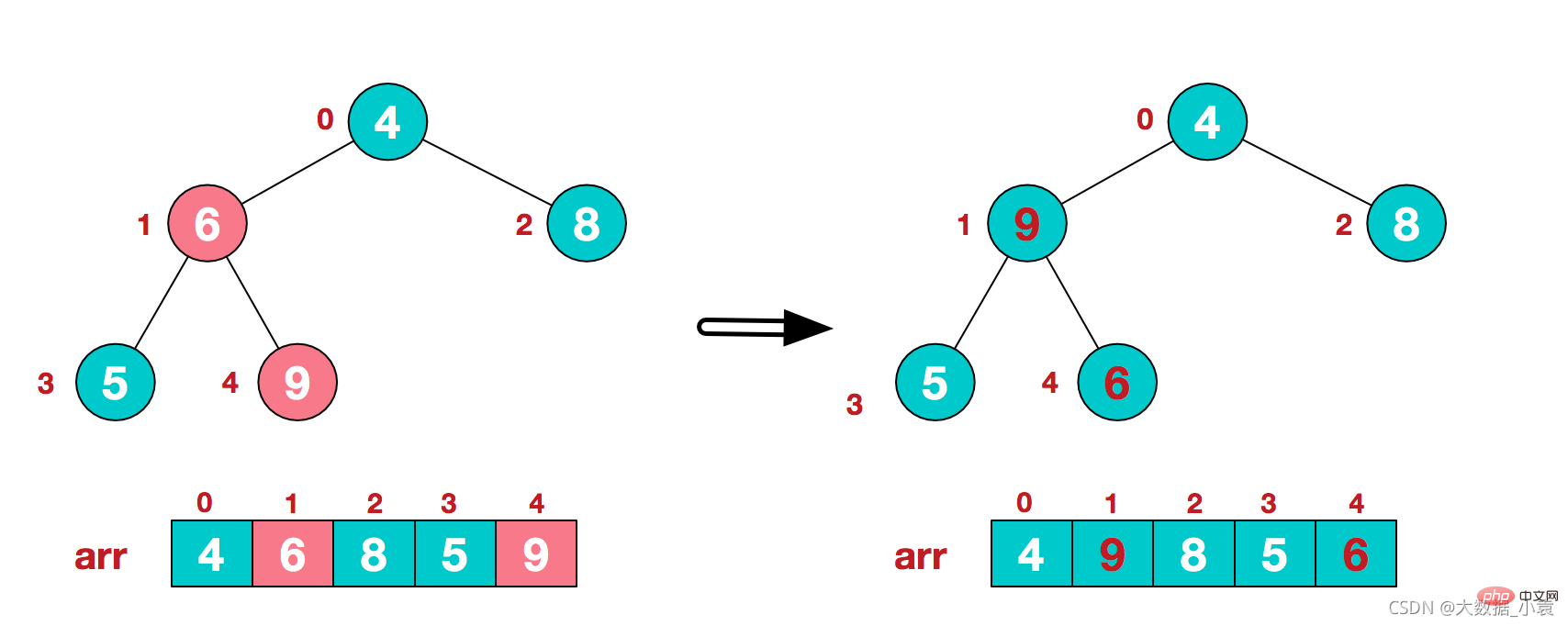
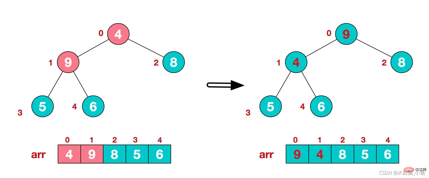 4)这时,交换导致了子根[4,5,6]结构混乱,继续调整,[4,5,6]中6最大,交换4和6。
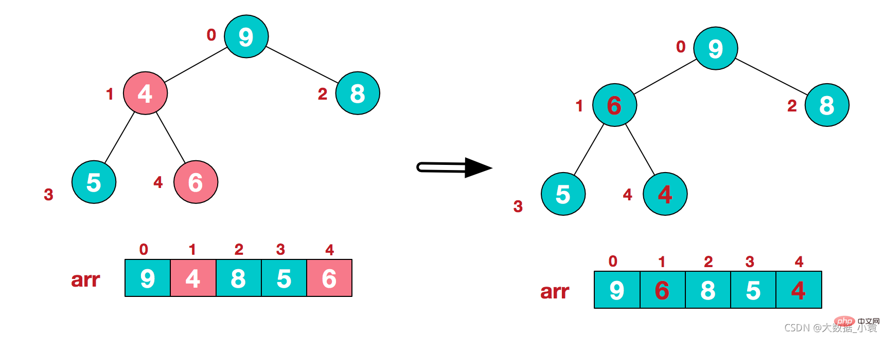 此时,我们就将一个无需序列构造成了一个大顶堆


The above is the detailed content of Detailed graphic explanation of Java data structures and algorithms. For more information, please follow other related articles on the PHP Chinese website!
Related articles
See more- Let you understand the JAVA reflection mechanism (summary sharing)
- How to get URL parameters in JavaScript? Detailed explanation of 4 common methods
- Take you to understand JavaScript destructuring assignment
- Summarize and organize the process control of JAVA learning
- A brief analysis of javascript data type learning Symbol type