


In this tutorial you will learn what a PivotTable is, find a number of examples showing how to create and use Pivot Tables in all version of Excel 365 through Excel 2007.
If you are working with large data sets in Excel, Pivot Table comes in really handy as a quick way to make an interactive summary from many records. Among other things, it can automatically sort and filter different subsets of data, count totals, calculate average as well as create cross tabulations.
Another benefit of using Pivot Tables is that you can set up and change the structure of your summary table simply by dragging and dropping the source table's columns. This rotation or pivoting gave the feature its name.
What is a Pivot Table in Excel?
An Excel Pivot Table is a tool to explore and summarize large amounts of data, analyze related totals and present summary reports designed to:
- Present large amounts of data in a user-friendly way.
- Summarize data by categories and subcategories.
- Filter, group, sort and conditionally format different subsets of data so that you can focus on the most relevant information.
- Rotate rows to columns or columns to rows (which is called "pivoting") to view different summaries of the source data.
- Subtotal and aggregate numeric data in the spreadsheet.
- Expand or collapse the levels of data and drill down to see the details behind any total.
- Present concise and attractive online of your data or printed reports.
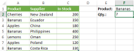
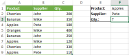
For example, you may have hundreds of entries in your worksheet with sales figures of local resellers:

One possible way to sum this long list of numbers by one or several conditions is to use formulas as demonstrated in SUMIF and SUMIFS tutorials. However, if you want to compare several facts about each figure, using a Pivot Table is a far more efficient way. In just a few mouse clicks, you can get a resilient and easily customizable summary table that totals the numbers by any field you want.

The screenshots above demonstrate just a few of many possible layouts. And the steps below show how you can quickly create your own Pivot Table in all versions of Excel.
Tip. The users of Excel 365 can also group and summarize data using a PIVOTBY formula. It's fully dynamic and updates in real time.
How to make a Pivot Table in Excel
Many people think that creating a Pivot Table is burdensome and time-consuming. But this is not true! Microsoft has been refining the technology for many years, and in the modern versions of Excel, the summary reports are user-friendly are incredibly fast. In fact, you can build your own summary table in just a couple of minutes. And here's how:
1. Organize your source data
Before creating a summary report, organize your data into rows and columns, and then convert your data range in to an Excel Table. To do this, select all of the data, go to the Insert tab and click Table.
Using an Excel Table for the source data gives you a very nice benefit - your data range becomes "dynamic". In this context, a dynamic range means that your table will automatically expand and shrink as you add or remove entries, so won't have to worry that your Pivot Table is missing the latest data.
Useful tips:
- Add unique, meaningful headings to your columns, they will turn into the field names later.
- Make sure your source table contains no blank rows or columns, and no subtotals.
- To make it easier to maintain your table, you can name your source table by switching to the Design tab and typing the name in the Table Name box the upper right corner of your worksheet.
2. Create a Pivot Table
Select any cell in the source data table, and then go to the Insert tab > Tables group > PivotTable.

This will open the Create PivotTable window. Make sure the correct table or range of cells is highlighted in the Table/Range field. Then choose the target location for your Excel Pivot Table:
- Selecting New Worksheet will place a table in a new worksheet starting at cell A1.
- Selecting Existing Worksheet will place your table at the specified location in an existing worksheet. In the Location box, click the Collapse Dialog button
to choose the first cell where you want to position your table.


Clicking OK creates a blank Pivot Table in the target location, which will look similar to this:

Useful tips:
- In most cases, it makse sense to place a Pivot Table in a separate worksheet, this is especially recommended for beginners.
- If you are creating a Pivot Table from the data in another worksheet or workbook, include the workbook and worksheet names using the following syntax [workbook_name]sheet_name!range, for example, [Book1.xlsx]Sheet1!$A$1:$E$20. Alternatively, you can click the Collapse Dialog button
and select a table or range of cells in another workbook using the mouse. - It might be useful to create a Pivot Table and Pivot Chart at the same time. To do this, in Excel 2013 and higher, go to the Insert tab > Charts group, click the arrow below the PivotChart button, and then click PivotChart & PivotTable. In Excel 2010 and 2007, click the arrow below PivotTable, and then click PivotChart.
3. Arrange the layout of your Pivot Table report
The area where you work with the fields of your summary report is called PivotTable Field List. It is located in the right-hand part of the worksheet and divided into the header and body sections:
- The Field Section contains the names of the fields that you can add to your table. The filed names correspond to the column names of your source table.
- The Layout Section contains the Report Filter area, Column Labels, Row Labels area, and the Values area. Here you can arrange and re-arrange the fields of your table.

The changes that you make in the PivotTable Field List are immediately reflected to your table.
How to add a field to Pivot Table
To add a field to the Layout section, select the check box next to the field name in the Field section.

By default, Microsoft Excel adds the fields to the Layout section in the following way:
- Non-numeric fields are added to the Row Labels area;
- Numeric fields are added to the Values area;
- Online Analytical Processing (OLAP) date and time hierarchies are added to the Column Labels area.
How to remove a field from a Pivot Table
To delete a certain field, you can either:
- Uncheck the box nest to the field's name in the Field section of the PivotTable pane.
- Right-click on the field in your Pivot Table, and then click "Remove Field_Name".

How to arrange Pivot Table fields
You can arrange the fields in the Layout section in three ways:
-
Drag and drop fields between the 4 areas of the Layout section using the mouse. Alternatively, click and hold the field name in the Field section, and then drag it to an area in the Layout section - this will remove the field from the current area in the Layout section and place it in the new area.
- Right-click the field name in the Field section, and then select the area where you want to add it:
- Click on the filed in the Layout section to select it. This will also display the options available for that particular field.


4. Choose summary function for Values (optional)
By default, Microsoft Excel applies the Sum function to numeric value fields placed in the Values area. Conversely, for non-numeric data (such as text, dates, or Boolean values), the Count function is automatically applied.
However, you are free to choose a different summary function according to your preference. For this, right-click on the value field you wish to modify, select Summarize Values By, and then choose the desired function from the options provided.
Below, you'll find an example of a Pivot Table utilizing the Averagefunction:

The functions' names are mostly self-explanatory:
- Sum - calculates the sum of the values.
- Count - counts the number of non-empty values (works as the COUNTA function).
- Average - calculates the average of the values.
- Max - finds the largest value.
- Min - finds the smallest value.
- Product - calculates the product of the values.
To get more specific functions, click Summarize Values By > More Options….
5. Show different calculations in value fields (optional)
Excel Pivot Tables provide one more useful feature that enables you to present values in different ways, for example show totals as percentage or rank values from smallest to largest and vice versa. The full list of calculation options is available here.
This feature is called Show Values As and it's accessible by right-clicking the field in the table in Excel 2013 and higher. In Excel 2010 and lower, you can also find this option on the Options tab, in the Calculations group.

Tip. The Show Values As feature may prove especially useful if you add the same field more than once and show, for example, total sales and sales as a percent of total at the same time. See an example of such a table.
This is how you create Pivot Tables in Excel. And now it's time for you to experiment with the fields a bit to choose the layout best suited for your data set.
Working with PivotTable Field List
The Pivot Table pane, which is formally called PivotTable Field List, is the main tool that you use to arrange your summary table exactly the way you want. To make your work with the fields more comfortable, you may want to customize the pane to your liking.
Changing the Field List view
If you want to change how the sections are displayed in the Field List, click the Tools button, and choose your preferred layout.

You can also resize the pane horizontally by dragging the bar (splitter) that separates the pane from the worksheet.
Closing and opening the PivotTable pane
Closing the PivotTableField List is as easy as clicking the Close button (X) in the top right corner of the pane.Making it to show up again is not so obvious :)
To display the Field List again, right-click anywhere in the table, and then select Show Field List from the context menu.

You can also click the Field List button on the Ribbon, which resides on the Analyze / Options tab, in the Show group.

Using Recommended PivotTables
As you have just seen, creating a Pivot Table in Excel is easy. However, the modern versions of Excel take even a step further and make it possible to automatically make a report most suited for your source data. All you have to do is 4 mouse clicks:
- Click any cell in your source range of cells or table.
- On the Insert tab, click Recommended PivotTables. Microsoft Excel will immediately display a few layouts, based on your data.
- In the Recommended PivotTables dialog box, click a layout to see its preview.
- If you are happy with the preview, click the OK button, and get a Pivot Table added to a new worksheet.

As you see in the screenshot above, Excel was able to suggest just a couple of basic layouts for my source data, which are far inferior to the Pivot Tables we created manually a moment ago. Of course, this is only my opinion and I am biased, you know : )
Overall, using the Recommended PivotTable is a quick way to get started, especially when you have a lot of data and are not sure where to start.
How to use Pivot Table in Excel
Now that you know the basics, you can navigate to the Analyze and Design tabs of the PivotTable Tools in Excel 2013 and higher, (Options and Design tabs in Excel 2010 and 2007) to explore the groups and options provided there. These tabs become available as soon as you click anywhere within your table.

You can also access options and features that are available for a specific element by right-clicking on it.
How to design and improve Pivot Table
Once you have created a Pivot Table based on your source data, you may want to refine it further to make powerful data analysis.
To improve the table's design, head over to the Design tab where you will find plenty of pre-defined styles. To create your own style, click the More button in the PivotTable Styles gallery, and then click "New PivotTable Style...".
To customize the layout of a certain field, click on that field, then click the Field Settings button on the Analyze tab in Excel 2013 and higher (Options tab in Excel 2010 and 2007). Alternatively, you can right click the field and choose Field Settings from the context menu.
The screenshot below demonstrate a new design and layout for our Pivot Table in Excel 2013.

How to get rid of "Row Labels" and "Column Labels" headings
When you are creating a Pivot Table, Excel applies the Compact layout by default. This layout displays "Row Labels" and "Column Labels" as the table headings. Agree, these aren't very meaningful headings, especially for novices.
An easy way to get rid of these ridiculous headings is to switch from the Compact layout to Outline or Tabular. To do this, go to the Design ribbon tab, click the Report Layout dropdown, and choose Show in Outline Form or Show in Tabular Form.

This will display the actual field names, as you see in the table on the right, which makes much more sense.

Another solution is to go to the Analyze (Options) tab, click the Options button, switch to the Display tab and uncheck the "Display Field Captions and Filter Dropdowns" box. However, this will remove all field captions as well as filter dropdowns in your table.
How to refresh a Pivot Table in Excel
Although a Pivot Table report is connected to your source data, you might be surprised to know that Excel does not refresh it automatically. You can get any data updates by performing a refresh operation manually, or have it refresh automatically when you open the workbook.
Refresh the Pivot Table data manually
- Click anywhere in your table.
- On the Analyze tab (Options tab in earlier versions), in the Data group, click the Refresh button, or press ALT F5.
Alternatively, you can right-click the table, and choose Refresh from the context menu.

To refresh all Pivot Tables in your workbook, click the Refresh button arrow, and then click Refresh All.
Note. If the format of your Pivot Table gets changed after refreshing, make sure the "Autofit column width on update" and "Preserve cell formatting on update" options are selected. To check this, click the Analyze (Options) tab > PivotTable group > Options button. In the PivotTable Options dialog box, switch to the Layout & Format tab and you will find these check boxes there.
After starting a refresh, you can review the status or cancel it if you've changed your mind. Just click on the Refresh button arrow, and then click either Refresh Status or Cancel Refresh.
Refreshing a Pivot Table automatically when opening the workbook
- On the Analyze / Options tab, in the PivotTable group, click Options > Options.
- In the PivotTable Options dialog box, go to the Data tab, and select the Refresh data when opening the file check box.

How to move a Pivot Table to a new location
If you want to move your table to a new workbook, worksheet are some other area in the current sheet, head over to the Analyze tab (Options tab in Excel 2010 and earlier) and click the Move PivotTable button in the Actions group. Select a new destination and click OK.

How to delete an Excel Pivot Table
If you no longer need a certain summary report, you can delete it in a number of ways.
- If your table resides in a separate worksheet, simply delete that sheet.
- If your table is located along with some other data on a sheet, select the entire Pivot Table using the mouse and press the Delete key.
- Click anywhere in the Pivot Table that you want to delete, go to the Analyze tab (Options tab in Excel 2010 and earlier) > Actions group, click the little arrow below the Select button, choose Entire PivotTable, and then press Delete.

Note. If any PivotTable chart is associated with your table, deleting the Pivot Table will turn it into a standard chart that can no longer be pivoted or updated.
How to prevent pivot table columns from resizing on every change or refresh
By default, Excel pivot tables automatically resize their columns to fit the contents whenever there's a change or refresh. This includes almost every action like adding or removing fields, filtering with drop-down menus, slicers and timelines, or making layout adjustments. While this automatic resizing can be helpful in some situations, it becomes really annoying when the worksheet contains other data outside the pivot table.
Thankfully, there's a simple setting to disable the auto-fit columns feature:
- Right-click any cell inside the pivot table.
- Choose PivotTable Options... from the context menu.
- On the Layout & Format tab, unselect the Autofit column widths on update checkbox.
- Press OK to confirm the change.

By following these steps, you can stop pivot table columns from automatically resizing with every change or refresh, providing a more stable and predictable layout for your Excel worksheets.
Pivot Table examples
The screenshots below demonstrate a few possible Pivot Table layouts for the same source data that might help you to get started on the right path. Feel free to download them get a hands-on experience.
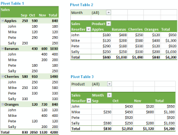
Pivot Table example 1: Two-dimensional table
- No Filter
- Rows: Product, Reseller
- Columns: Months
- Values: Sales

Pivot Table example 2: Three-dimensional table
- Filter: Month
- Rows: Reseller
- Columns: Product
- Values: Sales
This Pivot Table lets you filter the report by month.

Pivot Table example 3: One field is displayed twice - as total and % of total
- No Filter
- Rows: Product, Reseller
- Values: SUM of Sales, % of Sales
This summary report shows total sales and sales as a percent of total at the same time.

Hopefully, this Pivot Table tutorial has been a good starting point for you. If you want to learn advanced features and capabilities of Excel Pivot Tables, check out the links below. And thank you for reading!
Available downloads:
Pivot Table examples (.xlsx file)
The above is the detailed content of How to make and use Pivot Table in Excel. For more information, please follow other related articles on the PHP Chinese website!

 How to use SUMIF function in Excel with formula examplesMay 13, 2025 am 10:53 AM
This tutorial explains the Excel SUMIF function in plain English. The main focus is on real-life formula examples with all kinds of criteria including text, numbers, dates, wildcards, blanks and non-blanks. Microsoft Excel has a handful o
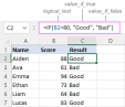 IF function in Excel: formula examples for text, numbers, dates, blanksMay 13, 2025 am 10:50 AM
In this article, you will learn how to build an Excel IF statement for different types of values as well as how to create multiple IF statements. IF is one of the most popular and useful functions in Excel. Generally, you use an IF statem
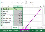 How to sum a column in Excel - 5 easy waysMay 13, 2025 am 09:53 AM
This tutorial shows how to sum a column in Excel 2010 - 2016. Try out 5 different ways to total columns: find the sum of the selected cells on the Status bar, use AutoSum in Excel to sum all or only filtered cells, employ the SUM function
 How to make and use Pivot Table in ExcelMay 13, 2025 am 09:36 AM
In this tutorial you will learn what a PivotTable is, find a number of examples showing how to create and use Pivot Tables in all version of Excel 365 through Excel 2007. If you are working with large data sets in Excel, Pivot Table comes
 Excel SUMIFS and SUMIF with multiple criteria – formula examplesMay 13, 2025 am 09:05 AM
This tutorial explains the difference between the SUMIF and SUMIFS functions in terms of their syntax and usage, and provides a number of formula examples to sum values with multiple AND / OR criteria in Excel 365, 2021, 2019, 2016, 2013,
 How You Can Use Wildcards in Microsoft Excel to Refine Your SearchMay 13, 2025 am 01:59 AM
Excel wildcards: a powerful tool for efficient search and filtering This article will dive into the power of wildcards in Microsoft Excel, including their application in search, formulas, and filters, and some details to note. Wildcards allow you to perform fuzzy matching, making it more flexible to find and process data. *Wildcards: asterisks () and question marks (?)** Excel mainly uses two wildcards: asterisk (*) and question mark (?). *Asterisk (): Any number of characters** The asterisk represents any number of characters, including zero characters. For example: *OK* Match the cell containing "OK", "OK&q
 Excel IF function with multiple conditionsMay 12, 2025 am 11:02 AM
The tutorial shows how to create multiple IF statements in Excel with AND as well as OR logic. Also, you will learn how to use IF together with other Excel functions. In the first part of our Excel IF tutorial, we looked at how to constru
 How to calculate percentage in Excel - formula examplesMay 12, 2025 am 10:28 AM
In this tutorial, you will lean a quick way to calculate percentages in Excel, find the basic percentage formula and a few more formulas for calculating percentage increase, percent of total and more. Calculating percentage is useful in m


Hot AI Tools

Undresser.AI Undress
AI-powered app for creating realistic nude photos

AI Clothes Remover
Online AI tool for removing clothes from photos.

Undress AI Tool
Undress images for free

Clothoff.io
AI clothes remover

Video Face Swap
Swap faces in any video effortlessly with our completely free AI face swap tool!

Hot Article
Hot Tools

MinGW - Minimalist GNU for Windows
This project is in the process of being migrated to osdn.net/projects/mingw, you can continue to follow us there. MinGW: A native Windows port of the GNU Compiler Collection (GCC), freely distributable import libraries and header files for building native Windows applications; includes extensions to the MSVC runtime to support C99 functionality. All MinGW software can run on 64-bit Windows platforms.

Dreamweaver Mac version
Visual web development tools

MantisBT
Mantis is an easy-to-deploy web-based defect tracking tool designed to aid in product defect tracking. It requires PHP, MySQL and a web server. Check out our demo and hosting services.

WebStorm Mac version
Useful JavaScript development tools

Zend Studio 13.0.1
Powerful PHP integrated development environment

