


In this article, we'll explore what a #NAME error is, why it occurs, and how to fix this error in Excel.
Even experienced Excel users may encounter errors while working with complex spreadsheets. One such error is #NAME, which can be frustrating to deal with but is usually easy to fix, especially when you know the reasons behind it.
What is a #NAME error in Excel?
#NAME? is a common Excel error notation that appears when a formula or function cannot find the referenced data it needs to complete the calculation. This could be caused by a few different things, such as a misspelling in the formula name or an invalid reference. It can also occur when a cell or range has been named incorrectly.

Reasons for #NAME error in Excel
There are several reasons why a #NAME? error may occur in Excel. Here are some of the most common ones.
Function name misspelled
One of the most common causes of a #NAME error in Excel is the incorrect spelling of a function's name. Microsoft Excel has a large library of built-in functions that allow users to perform a variety of calculations. However, if the function's name is typed incorrectly, Excel will be unable to identify it and will display the #NAME error.
For instance, let's say you need to use a XLOOKUP or VLOOKUP formula to retrieve data from a table. If you accidentally misspell the function name as XLOKUP or VLOKUP, Excel won't recognize it as a valid function, resulting in a #NAME error being returned.

Using new functions in older Excel versions
Another frequent cause of a #NAME error in Excel is trying to use new functions in earlier versions. Microsoft frequently updates Excel by adding new features and functions, but these updates are not backward compatible.
For example, all the dynamic array functions such as UNIQUE, FILTER, SORT, and others introduced in Excel 365 are not available in older versions. If you try to use any of those functions in Excel 2019 and earlier, you will get a #NAME error.

To avoid this issue, check the compatibility of the function with your Excel and upgrade to a newer version if necessary.
Invalid named range
Excel uses named ranges, which are user-defined labels for cells or ranges, to make it easier to reference data in formulas. When a formula refers to a named range that doesn't exist or has been deleted, Excel returns a #NAME error.
A misspelled named range can also lead to a #NAME error. For example, if you named a range Items but accidentally typed Itms in a formula, a #NAME error will occur.

One more source of errors related to named ranges can be the scope of a named range. Excel names can have either local scope (defined within a worksheet) or global scope (defined across the entire workbook). If you encounter a #NAME error when referencing a valid named range, it is likely because the range is scoped locally to a different sheet. To resolve this, ensure that you are referencing the named range correctly and that it has the appropriate scope. Read more about Excel names scope.
Incorrect range reference
Incorrectly referencing a range in a formula is yet another common cause of a #NAME error in Excel. This can happen if you manually enter the range reference and make a mistake. Some common mistakes when entering range references include:
- Omitting a colon, such as typing A1A10 instead of A1:A10.
- Incorrect address of the starting or ending cell reference, such as AS:A20 instead of A4:A20.
- Referencing a cell outside the valid Excel range of A1:XFD1048576.

To avoid typos, it's always best to select a range using a mouse or use Excel's built-in range selection tools.
Missing quotation marks around text values
When using text values in Excel formulas, you need to enclose text in double quotation marks, whether your value includes letters, special characters or only a space. Entering a text value without double quotes confuses Excel as it interprets the value as a function or range name, resulting in a #NAME error if no match is found.
For example, this CONCAT formula works nicely:
=CONCAT("Today is "&TEXT(TODAY(),"mmmm d, yyyy"))
While this one causes a #NAME error:
=CONCAT(Today is &TEXT(TODAY(),"mmmm d, yyyy"))

Using smart quotes (also known as curly quotes) instead of straight quotes can also result in a #NAME error in Excel formulas. This error typically occurs when copying a formula from the web or another external source.
For example, if you copy the following formula to your worksheet, Excel will not recognize the smart quotes and will return a #NAME error:
=CONCAT(“Today is ”&TEXT(TODAY(),"mmmm d, yyyy")),
Once you replace the smart quotes with straight quotes, the formula will work correctly. It's always a good practice to check for smart quotes and replace them with straight quotes when copying a formula from somewhere.
Specific add-in or custom function missing
You may also encounter the #NAME? error if a particular add-in is required to execute a formula and that add-in is not installed or enabled in your Excel.
For example, to use the EUROCONVERT function, the Euro Currency Tools add-in needs to be enabled. To activate it, this is what you need to do:
- Click File > Options > Add-ins.
- In the Manage list box, pick Excel Add-ins and click Go.
- Check the corresponding box and click OK.
Aside from missing add-ins, a #NAME error can also be caused by a custom function missing in a specific sheet. Let's say you created a user-defined function named FindSumCombinations to find all combinations that equal a given sum, which works beautifully in the sheet where the function's code is added. In the sheet where the code is missing, a #NAME error occurs.

How to avoid #NAME error in Excel
Now that we have covered some of the most common reasons for the #NAME error in Excel and how to troubleshoot them, let's have a look at some tips that can help you prevent this error in the first place :)
Excel Formula AutoComplete
After you start typing a formula in a cell, Excel shows a drop-down list of matching functions and names. This feature is known as Formula AutoComplete. By selecting the function or name from the list, you can avoid manually typing the full formula and prevent misspelling the function name. Additionally, the formula assistant offers a brief explanation of the function's syntax, making it easier for you to use the function correctly.

Formula Wizard
The Formula Wizard in Excel can guide you through the process of building a formula step-by-step, ensuring that you use the correct function arguments and enter the correct references.
Name Manager and Use in Formula
Lastly, use the Name Manager to keep track of your defined names. This tool allows you to view and edit all named ranges in your workbook, ensuring that they are correct and up-to-date. By keeping your named ranges organized, you can avoid typo mistakes and scope mismatches that lead to the #NAME error.
If you need to use a specific named range in a formula but are unsure about its exact name, you can easily find it using the Use in Formula option located on the Formula tab, in the Defined Names group. Clicking on it will display a list of all the defined names in the current workbook, and you can select the right one with a click.

How to find #NAME errors in Excel
If you are facing the #NAME error in your worksheet, it's important to quickly identify all the cells that contain this error so you can fix them. This section shows a couple of methods to quickly do this.
Select #NAME errors with Go To Special
Using this feature, you can quickly select all the cells in the current sheet that have an error.
- Select the range of cells you want to check.
- On the Home tab, in the Editing group, click Find & Select > Go to Special. Or press F5 and click Special… .
- In the dialog box that appears, select Formulas and check the box for Errors.
- Click OK.

As a result, Excel will select all cells within a specified range that contain errors, including #NAME. Once the errors are identified, you can fix them by using the correct function name, correcting the named range reference, or addressing any other issue causing the error.
Note. This feature is not specific to the #NAME error – it will select cells with any type of error.
Find and remove all #NAME errors using Find and Replace
Another option to find #NAME errors in Excel is to use the Find and Replace functionality. The steps are:
- Select the range of cells you want to search for #NAME errors.
- Press the Ctrl F shortcut to open the Find and Replace dialog box.
- In the Find what field, type #NAME?.
- Click on the Options button to expand the dialog box.
- In the Look in drop-down box, select Values.
- Click the Find All button.
Excel will display a list of all the cells that contain the #NAME error. Here, you can select a specific item to navigate to the corresponding cell and fix the error. Or you can select multiple items to highlight all the cells in the worksheet or delete all errors in one go.

Tip. To get rid of all #NAME errors at a time, you can use the Replace All feature. Simply press Ctrl H on your keyboard to open the Find and Replace dialog box. Then, type #NAME? in the Find what box, leave the Replace with box blank and click Replace All. This will remove all instances of the #NAME error in your worksheet.
That's how to find and correct the #NAME error in Excel. By understanding the reasons behind it and using the tips provided in this article, you can minimize the risk of encountering this error in your work and save time and effort in fixing it.
Practice workbook for download
#NAME error in Excel - examples (.xlsx file)
The above is the detailed content of #NAME error in Excel: reasons and fixes. For more information, please follow other related articles on the PHP Chinese website!

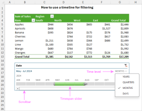 How to create timeline in Excel to filter pivot tables and chartsMar 22, 2025 am 11:20 AM
This article will guide you through the process of creating a timeline for Excel pivot tables and charts and demonstrate how you can use it to interact with your data in a dynamic and engaging way. You've got your data organized in a pivo
 how to sum a column in excelMar 14, 2025 pm 02:42 PM
The article discusses methods to sum columns in Excel using the SUM function, AutoSum feature, and how to sum specific cells.
 how to do a drop down in excelMar 12, 2025 am 11:53 AM
This article explains how to create drop-down lists in Excel using data validation, including single and dependent lists. It details the process, offers solutions for common scenarios, and discusses limitations such as data entry restrictions and pe
 how to make pie chart in excelMar 14, 2025 pm 03:32 PM
The article details steps to create and customize pie charts in Excel, focusing on data preparation, chart insertion, and personalization options for enhanced visual analysis.
 how to make a table in excelMar 14, 2025 pm 02:53 PM
Article discusses creating, formatting, and customizing tables in Excel, and using functions like SUM, AVERAGE, and PivotTables for data analysis.
 how to calculate mean in excelMar 14, 2025 pm 03:33 PM
Article discusses calculating mean in Excel using AVERAGE function. Main issue is how to efficiently use this function for different data sets.(158 characters)
 how to add drop down in excelMar 14, 2025 pm 02:51 PM
Article discusses creating, editing, and removing drop-down lists in Excel using data validation. Main issue: how to manage drop-down lists effectively.
 All you need to know to sort any data in Google SheetsMar 22, 2025 am 10:47 AM
Mastering Google Sheets Sorting: A Comprehensive Guide Sorting data in Google Sheets needn't be complex. This guide covers various techniques, from sorting entire sheets to specific ranges, by color, date, and multiple columns. Whether you're a novi


Hot AI Tools

Undresser.AI Undress
AI-powered app for creating realistic nude photos

AI Clothes Remover
Online AI tool for removing clothes from photos.

Undress AI Tool
Undress images for free

Clothoff.io
AI clothes remover

AI Hentai Generator
Generate AI Hentai for free.

Hot Article
Hot Tools

VSCode Windows 64-bit Download
A free and powerful IDE editor launched by Microsoft

SublimeText3 Mac version
God-level code editing software (SublimeText3)

MantisBT
Mantis is an easy-to-deploy web-based defect tracking tool designed to aid in product defect tracking. It requires PHP, MySQL and a web server. Check out our demo and hosting services.

Notepad++7.3.1
Easy-to-use and free code editor

SAP NetWeaver Server Adapter for Eclipse
Integrate Eclipse with SAP NetWeaver application server.

