


This article will guide you through the process of creating a timeline for Excel pivot tables and charts and demonstrate how you can use it to interact with your data in a dynamic and engaging way.
You've got your data organized in a pivot table and are ready to dig in, but there is a catch – it has a time element. Maybe it's sales figures over months or project deadlines scattered throughout the year. How do you make sense of it all without drowning in numbers? The answer is timelines!
What is a timeline in Excel pivot tables and charts?
Timeline in an Excel PivotTable or PivotChart is an interactive tool that lets you quickly filter data by time periods using a slider control. Timelines are available for pivot tables and pivot charts that have a date field in the rows or columns area. They can be used to filter data by years, quarters, months, or days, and can be formatted to match the style of your workbook.

Picture this: you've got your pivot table or chart set up, but instead of scrolling through endless rows of dates or fiddling with filters, you've got this neat little slider right in front of you. That's your timeline! This nifty tool lets you zoom in and out of specific time periods with just a few clicks, making it super easy to focus on the data that matters most. They are fully dynamic, meaning you can adjust the timeframe on the fly and your pivot table and graph will instantly update to reflect the changes.
How to create a timeline for Excel pivot table
It's very quick to make a pivot table timeline in Excel. Just follow these steps:
- Click anywhere in the pivot table to activate its ribbon tabs.
- On the PivotTable Analyze tab, in the Filter group, click the Insert Timeline button.
- In the dialog box that pops up, select the date field you want to include.
- Once you've made your selection, hit the OK button.
And just like that, you've successfully added a timeline to your Excel pivot table! Now you can easily filter and examine your data by time periods, revealing useful insights with no trouble.

Tips and notes:
- To insert a timeline, a date field doesn't necessarily have to be displayed within the pivot table. However, the source dataset must contain at least one column with date/time values. These values serve as the foundation for the timeline functionality, even if they are not directly visible in the pivot table itself.
- To add multiple timelines at once, select two or more date/time fields in the dialog box. Each selected field will produce its own separate dynamic filter.
How to make a timeline for Excel pivot chart
When you make a timeline for an Excel pivot table, it gets automatically connected to all pivot charts based on that table. If you wish to incorporate a timeline directly into the pivot chart area, follow these steps:
- Click on your pivot chart to ensure it's selected.
- Navigate to the PivotChart Analyze tab and click Insert Timeline.
- Select the target date field and click OK. This will insert the timeline in the worksheet.
- Resize the chart area as needed by dragging the borders. You can make the chart area bigger and the plot area smaller to accommodate the timeline.
- Drag the timeline into the empty space at the bottom of the chart area.
The result might look something like this:

How to use a timeline in Excel
Once you have set up your timeline, you can use it to filter your pivot table and chart by time period.
- Select time level – utilize the Time Level dropdown menu to choose the desired time, whether it's years, quarters, months, or days.
- Pick the period – Use the timespan slider to select your preferred time interval. To choose a single period, simply click on the corresponding tile. For selecting multiple days, months, quarters, or years in sequence, click on one tile, then drag the timespan handles to adjust the date range on either or both sides.
- Scroll through periods - navigate through different time periods by dragging the scrollbar to the desired position.

Tip. To prevent pivot table columns from resizing when using a timeline, turn off the Autofit column widths on update feature.
How to customize Excel timeline
To make your data analysis even better, you have the flexibility to fine-tune the default timeline created by Excel. By changing its appearance, position, and size, you can get the dynamic filter to perfectly complement your pivot table or chart.
Move a timeline
To relocate the timeline to a more suitable position, simply drag it as you would any other object in the sheet:
- Hover the cursor over the upper part of the timeline until the four-pointed arrow appears, indicating that the timeline is ready to be moved.
- Click and drag the timeline to your desired location.

Resize a timeline
To quickly change the size of the timeline, click it, and then drag the sizing handles to the size you want.
Alternatively, you can set the desired height and width in this way:
- Select the timeline.
- On the Timeline tab, in the Size group, set the height and width in the corresponding boxes.

Change timeline style
You can make your timeline better suited to your presentation needs by customizing its style. With 12 pre-defined styles and the ability to design your own, you have plenty of options to get the desired look.
Here are the steps to change the timeline style:
- Select the timeline to activate its ribbon tab.
- On the Timeline tab, pick the style you want from the Timeline Styles gallery.
- Alternatively, click New Timeline Style to create your own unique style.
With these options, you can easily modify the appearance of your timespan slider to suit your preferences and make your data analysis more engaging to look at.

Change timeline caption
By default, the caption name of an Excel timeline mirrors the name of the corresponding date column. However, you can customize it at any time using the following steps:
- Select the timeline by clicking on it.
- Navigate to the Timeline tab.
- In the Timeline Caption box, enter the desired name for the caption.
- Press Enter to confirm the change.
With these simple steps, you can personalize the timeline caption to better reflect its context or purpose.

Hide or show the selection label
By default, the date range currently included in the filter is displayed in the upper-left corner of the timeline. You can control its visibility using the Selection Label option located in the Timeline tab, within the Show group. To hide the filtered date range, uncheck this checkbox. To make it visible again, just re-select the checkbox.

How to lock the timeline position in a sheet
To ensure that the position of a timeline remains fixed within a sheet, follow these steps:
- Right-click on the timeline, and then select Size and Properties… from the context menu.
- In the Format Timeline pane, navigate to the Properties section, and check the Don't move or size with cells option.
This way, your dynamic filter will stay in place even as you add or delete rows and columns, adjust fields in the pivot table, or make other modifications.

How to connect a timeline to multiple pivot tables
If you have several PivotTables based on the same data source, you can use a single timeline to filter those multiple tables simultaneously. To link a timeline to more than one table, follow these steps:
- Select the timeline by clicking on it.
- Go to the Timeline tab and click Report Connections. Alternatively, right-clink the timeline and choose Report Connections from the context menu.
- In the Report Connections dialog box, select the PivotTables you want to filter.
To disconnect the timeline from a specific table, uncheck the box next to its name.

Tip. If you wish to filter the same date field using both a timeline and slicers, you can do so by enabling the Allow multiple filters per field feature. To access this option, right-click on the pivot table and select PivotTable Options from the context menu. In the dialog box that opens, switch to the Totals & Filters tab and check the Allow multiple filters per field box.
How to clear timeline filter
To clear a timeline, click the Clear Filter button or press the Alt + C shortcut. This will remove all applied filters and reset the timeline, allowing for a fresh analysis of the data.

How to remove a timeline
After using your filter slider for a while, you may not want it anymore. To delete the timeline from your Excel sheet, you can do any of the following:
- Right-click the timeline and choose Remove Timeline from the context menu.
- Select the timeline and press the Delete key on the keyboard.
Either way, the timeline will be promptly removed from your work sheet, letting you focus on other aspects of your analysis.

Tip. If you accidentally deleted the timeline, don't worry. You can easily bring it back using the Undo feature. Simply press Ctrl + Z or use the Undo button to revert the deletion.
Excel pivot table timeline not working
Encountering an error while trying to insert a timeline for a PivotTable or PivotChart in Excel? You might see a message stating: "We can't create a Timeline for this report because it doesn't have a field formatted as Date" even though your dataset does have a date column.

There are two potential reasons for a pivot table timeline not working:
- Your source dataset lacks a date column altogether.
- Your dataset does have a date column, but the values are stored as text strings that only resemble dates.
To resolve the error, you must either include a column of actual dates or convert the existing text values into dates. Here are some tips to differentiate between normal Excel dates and text-dates, along with quick methods to convert text to date format.
In conclusion, using timelines in Excel pivot tables and charts unlocks a whole new dimension of data analysis. With just a few clicks, they can turn static information into dynamic insights, helping you make smarter decisions faster. So, try it out, experiment, and see how your data comes to life before your eyes.
Practice workbook for download
Excel Timeline - examples (.xlsx file)
The above is the detailed content of How to create timeline in Excel to filter pivot tables and charts. For more information, please follow other related articles on the PHP Chinese website!

 MEDIAN formula in Excel - practical examplesApr 11, 2025 pm 12:08 PM
This tutorial explains how to calculate the median of numerical data in Excel using the MEDIAN function. The median, a key measure of central tendency, identifies the middle value in a dataset, offering a more robust representation of central tenden
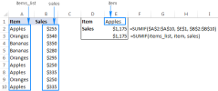
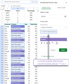 Google Spreadsheet COUNTIF function with formula examplesApr 11, 2025 pm 12:03 PM
Master Google Sheets COUNTIF: A Comprehensive Guide This guide explores the versatile COUNTIF function in Google Sheets, demonstrating its applications beyond simple cell counting. We'll cover various scenarios, from exact and partial matches to han
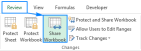 Excel shared workbook: How to share Excel file for multiple usersApr 11, 2025 am 11:58 AM
This tutorial provides a comprehensive guide to sharing Excel workbooks, covering various methods, access control, and conflict resolution. Modern Excel versions (2010, 2013, 2016, and later) simplify collaborative editing, eliminating the need to m
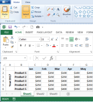 How to convert Excel to JPG - save .xls or .xlsx as image fileApr 11, 2025 am 11:31 AM
This tutorial explores various methods for converting .xls files to .jpg images, encompassing both built-in Windows tools and free online converters. Need to create a presentation, share spreadsheet data securely, or design a document? Converting yo
 Excel names and named ranges: how to define and use in formulasApr 11, 2025 am 11:13 AM
This tutorial clarifies the function of Excel names and demonstrates how to define names for cells, ranges, constants, or formulas. It also covers editing, filtering, and deleting defined names. Excel names, while incredibly useful, are often overlo
 Standard deviation Excel: functions and formula examplesApr 11, 2025 am 11:01 AM
This tutorial clarifies the distinction between standard deviation and standard error of the mean, guiding you on the optimal Excel functions for standard deviation calculations. In descriptive statistics, the mean and standard deviation are intrinsi
 Square root in Excel: SQRT function and other waysApr 11, 2025 am 10:34 AM
This Excel tutorial demonstrates how to calculate square roots and nth roots. Finding the square root is a common mathematical operation, and Excel offers several methods. Methods for Calculating Square Roots in Excel: Using the SQRT Function: The
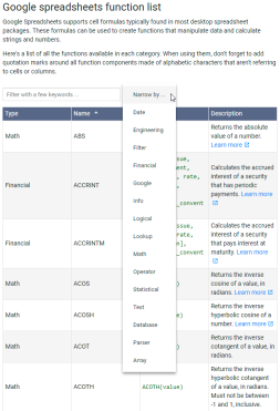 Google Sheets basics: Learn how to work with Google SpreadsheetsApr 11, 2025 am 10:23 AM
Unlock the Power of Google Sheets: A Beginner's Guide This tutorial introduces the fundamentals of Google Sheets, a powerful and versatile alternative to MS Excel. Learn how to effortlessly manage spreadsheets, leverage key features, and collaborate


Hot AI Tools

Undresser.AI Undress
AI-powered app for creating realistic nude photos

AI Clothes Remover
Online AI tool for removing clothes from photos.

Undress AI Tool
Undress images for free

Clothoff.io
AI clothes remover

Video Face Swap
Swap faces in any video effortlessly with our completely free AI face swap tool!

Hot Article
Hot Tools

PhpStorm Mac version
The latest (2018.2.1) professional PHP integrated development tool

SublimeText3 English version
Recommended: Win version, supports code prompts!

mPDF
mPDF is a PHP library that can generate PDF files from UTF-8 encoded HTML. The original author, Ian Back, wrote mPDF to output PDF files "on the fly" from his website and handle different languages. It is slower than original scripts like HTML2FPDF and produces larger files when using Unicode fonts, but supports CSS styles etc. and has a lot of enhancements. Supports almost all languages, including RTL (Arabic and Hebrew) and CJK (Chinese, Japanese and Korean). Supports nested block-level elements (such as P, DIV),

MinGW - Minimalist GNU for Windows
This project is in the process of being migrated to osdn.net/projects/mingw, you can continue to follow us there. MinGW: A native Windows port of the GNU Compiler Collection (GCC), freely distributable import libraries and header files for building native Windows applications; includes extensions to the MSVC runtime to support C99 functionality. All MinGW software can run on 64-bit Windows platforms.

Dreamweaver CS6
Visual web development tools

