


Quick guide to DGET functions: Efficiently extract single data values
- DGET Syntax
- Example 1: Single condition
- Example 2: Multiple Conditions
- Advantages of using DGET
- Disadvantages of using DGET
DGET function is a simple lookup function that retrieves a single value from a column in a table or database. It is especially suitable for extracting individual data points from large spreadsheets, avoiding endless scrolling to find the required information.
This guide will walk you through the syntax of the function, show some practical examples, and discuss its pros and cons.
DGET function syntax
The following is the syntax of this function:
<code>=DGET(a,b,c)</code>
Of:
- a is a database - a range of cells (including column headers), from which the formula will retrieve data. The database must be presented in such a way that the category (such as name, address, and age) is in the column and the data (record) is in the row.
- b is a field—Excel will use to search for the output column category label. This can be a word or a word string enclosed in double quotes (DGET is case-insensitive), or a cell reference.
- c is a condition - a range of cells that contain the search criteria.
All three parameters of this function are required, which means that if you omit any parameters, Excel will return a #VALUE! error.
To explain this more clearly, here are some examples.
Example 1: Single condition
Let's start with this very basic example, a list of employee IDs, names, departments and years of service.
Spreadsheet Settings
The blue table above is my search form, and the green table below is my database. The goal is to return the employee's name, department, and years of service in the blue search form when entering the employee ID to cell A2.

Before showing you how to pull data from a green database table to a blue search table, let me highlight some of the important things in the screenshot above:
- In my green database table, each column is a different category and each row is a different record.
- Both the database and the search table contain the same title.
- Because every employee has a unique ID, I know that the DGET function does not return a #NUM! error.
Add drop-down list
To avoid having to type the employee's ID in cell A2 every time, I will create a drop-down list of these numbers.
If you want to do the same, select the relevant cell and click Data Verification in the Data tab. Then, select List in the Allow field and select the cell that contains the drop-down data in the Source field. In my example, even though I have only 175 IDs in my database, I have expanded the data validation list to cell A236 so that I can add any other IDs to my dropdown list.

Note that cell A2 now contains a drop-down arrow that can be clicked to display the full list of IDs.

After selecting one of the IDs, I can start my DGET search.
DGET formula
In cell B2, I will type:
<code>=DGET(a,b,c)</code>
Because cells A4 to E172 represent my database, the value (name) in B1 is the category or field I want Excel to search for, while cells A1 and A2 (category name "ID" and from my drop-down list ID in cell A2 selected) is the condition. When I press Enter, I can see that Excel has successfully retrieved the name based on the ID in cell A2.

parameters a and c include the dollar sign ($) before the column and row references because they are absolute references. In other words, these references will never change - I will always use the ID to create the lookup and the database will always be in these cells. I added these dollar signs by pressing F4 after adding each reference to the formula.
However, I deliberately kept the parameter b as a relative reference, because I will now use Excel's fill handle to apply the same formula to the rest of the categories (last name, department, and service in my search table Year).

Note how the formula in cell E2 thus retrieves the field name from cell E1 while the database and conditional references remain unchanged.

I can now use the dropdown list I created to select a different ID in cell A2 to retrieve details of other employees.
If you format the database using Excel's table formatting tool, the parameter a will be the name of the table (also known as a structured reference), rather than its cell reference.
Example 2: Multiple Conditions
To make the lookup more specific - this is useful if you keep returning a #NUM! error due to multiple matches - you can use multiple conditions in the parameter c.
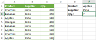
Here, I want to return to the ID, first and last name of the employee who I know have worked in the Personnel Department for ten years but I don’t quite remember my first name.

First, in cell A2, I will type:
<code>=DGET(a,b,c)</code>
Where cells A4 to A172 contain my database, cell A1 is the category, and cell D1 to E2 contains my two conditions. In fact, Excel creates an AND logical sequence between cells D2 and E2 to define my conditions.

Because I fixed the database and conditional references, but kept the category references as relative references, I could copy the formula into the rest of the cells in the search table to remind myself to remember the employee's name.

If you are more familiar with VLOOKUP, you may have noticed that you can use DGET to retrieve data from the right or left of the input formula, which is the flexibility VLOOKUP does not provide.
You can also create an OR logical sequence by adding another row to the search table. For example, if I know someone has been hired for 1 or 2 years, but I can't remember their name, I will type 1 in cell E2, 2 in cell E3, and put the parameter c Expand to cells E1 to E3. Excel then finds and returns entries with service years of 1 or 2. However, if multiple people meet these conditions, Excel returns a #NUM! error.
Properties of using DGET
You may be wondering, "Why should I use DGET when there are other more advanced functions?" Well, here are some of the benefits of using this tool:
- DGET has only three parameters, making it easier to use than other Excel find functions.
- DGET function is an old-fashioned tool! This means that unlike some of the more modern counterparts like XLOOKUP, it is compatible with older versions of Excel.
- DGET can return the value to the left of the search column when VLOOKUP can only perform right-looking searches.
- DGET will immediately adapt to changes in conditions.
- This function can be used with text and numbers.
Disadvantages of using DGET
On the other hand, while DGET's simplicity makes it easy to use, it also means some disadvantages to be noted:
| DGET 缺点 | 如何解决 |
|---|---|
| 一次只能查找一条记录。每次查找都需要其自己的标题和条件。 | 使用 XLOOKUP(如果返回数组位于查找数组的右侧,则使用 VLOOKUP),或为多个搜索创建单独的 DGET 检索区域。 |
| 如果有多个匹配项,DGET 将返回 #NUM! 错误。 | 修改数据,使其没有重复项,或使用 VLOOKUP,它将返回找到的第一个匹配值的数。 |
| DGET 不适用于水平表(类别位于行中,数据位于列中)。 | 使用 Excel 的转置工具翻转数据库的结构,使用专为适应水平表而设计的 HLOOKUP,或使用可以搜索任何方向的 XLOOKUP。 |
In this article, I discuss DGET, VLOOKUP, HLOOKUP, and XLOOKUP, some of the most famous lookup functions in Excel. But if I don't mention INDEX and MATCH, it would be too negligent because – when used in combination – they are powerful, flexible and adaptable alternatives.
The above is the detailed content of How to Use the DGET Function in Excel. For more information, please follow other related articles on the PHP Chinese website!

 How to use SUMIF function in Excel with formula examplesMay 13, 2025 am 10:53 AM
This tutorial explains the Excel SUMIF function in plain English. The main focus is on real-life formula examples with all kinds of criteria including text, numbers, dates, wildcards, blanks and non-blanks. Microsoft Excel has a handful o
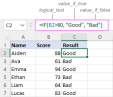 IF function in Excel: formula examples for text, numbers, dates, blanksMay 13, 2025 am 10:50 AM
In this article, you will learn how to build an Excel IF statement for different types of values as well as how to create multiple IF statements. IF is one of the most popular and useful functions in Excel. Generally, you use an IF statem
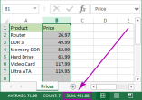 How to sum a column in Excel - 5 easy waysMay 13, 2025 am 09:53 AM
This tutorial shows how to sum a column in Excel 2010 - 2016. Try out 5 different ways to total columns: find the sum of the selected cells on the Status bar, use AutoSum in Excel to sum all or only filtered cells, employ the SUM function
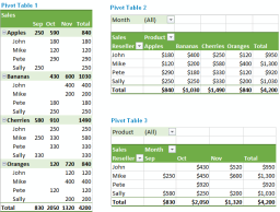 How to make and use Pivot Table in ExcelMay 13, 2025 am 09:36 AM
In this tutorial you will learn what a PivotTable is, find a number of examples showing how to create and use Pivot Tables in all version of Excel 365 through Excel 2007. If you are working with large data sets in Excel, Pivot Table comes
 Excel SUMIFS and SUMIF with multiple criteria – formula examplesMay 13, 2025 am 09:05 AM
This tutorial explains the difference between the SUMIF and SUMIFS functions in terms of their syntax and usage, and provides a number of formula examples to sum values with multiple AND / OR criteria in Excel 365, 2021, 2019, 2016, 2013,
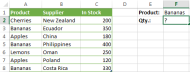
 How You Can Use Wildcards in Microsoft Excel to Refine Your SearchMay 13, 2025 am 01:59 AM
Excel wildcards: a powerful tool for efficient search and filtering This article will dive into the power of wildcards in Microsoft Excel, including their application in search, formulas, and filters, and some details to note. Wildcards allow you to perform fuzzy matching, making it more flexible to find and process data. *Wildcards: asterisks () and question marks (?)** Excel mainly uses two wildcards: asterisk (*) and question mark (?). *Asterisk (): Any number of characters** The asterisk represents any number of characters, including zero characters. For example: *OK* Match the cell containing "OK", "OK&q
 Excel IF function with multiple conditionsMay 12, 2025 am 11:02 AM
The tutorial shows how to create multiple IF statements in Excel with AND as well as OR logic. Also, you will learn how to use IF together with other Excel functions. In the first part of our Excel IF tutorial, we looked at how to constru
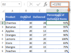 How to calculate percentage in Excel - formula examplesMay 12, 2025 am 10:28 AM
In this tutorial, you will lean a quick way to calculate percentages in Excel, find the basic percentage formula and a few more formulas for calculating percentage increase, percent of total and more. Calculating percentage is useful in m


Hot AI Tools

Undresser.AI Undress
AI-powered app for creating realistic nude photos

AI Clothes Remover
Online AI tool for removing clothes from photos.

Undress AI Tool
Undress images for free

Clothoff.io
AI clothes remover

Video Face Swap
Swap faces in any video effortlessly with our completely free AI face swap tool!

Hot Article
Hot Tools

Dreamweaver Mac version
Visual web development tools

ZendStudio 13.5.1 Mac
Powerful PHP integrated development environment

Notepad++7.3.1
Easy-to-use and free code editor

WebStorm Mac version
Useful JavaScript development tools

SAP NetWeaver Server Adapter for Eclipse
Integrate Eclipse with SAP NetWeaver application server.

