


嘿,Python爱好者!您是否希望以超音速速度运行Numpy代码?认识JAX!。您在机器学习,深度学习和数字计算过程中的新最好的朋友。将其视为具有超能力的Numpy。它可以自动处理梯度,编译代码以使用JIT快速运行,甚至可以在GPU和TPU上运行而不会破坏汗水。无论您是构建神经网络,处理科学数据,调整变压器模型,还是只是试图加快计算速度,JAX都会支持您。让我们深入研究,看看是什么使Jax如此特别。
本指南详细介绍了JAX及其生态系统。
学习目标
- 解释JAX的核心原理及其与Numpy的不同。
- 应用JAX的三个关键转换来优化Python代码。将Numpy操作转换为有效的JAX实现。
- 在JAX代码中识别并修复常见的性能瓶颈。在避免典型的陷阱的同时,正确实施JIT编译。
- 使用JAX从头开始构建和训练神经网络。使用JAX的功能方法实施常见的机器学习操作。
- 使用JAX的自动分化解决优化问题。执行有效的矩阵操作和数值计算。
- 将有效的调试策略应用于特定问题。实施用于大规模计算的内存效率模式。
本文作为数据科学博客马拉松的一部分发表。
目录
- 什么是JAX?
- Jax为什么脱颖而出?
- Jax入门
- 为什么要学习JAX?
- 基本的JAX转换
- 用JAX构建神经网络
- 最佳实践和技巧
- 性能优化
- 调试策略
- jax中的常见模式和成语
- 接下来是什么?
- 结论
- 常见问题
什么是JAX?
根据官方文档,JAX是用于加速阵列计算和程序转换的Python库,专为高性能数值计算和大规模机器学习而设计。因此,JAX本质上是类固醇上的Numpy,它将熟悉的Numpy风格操作与自动分化和硬件加速相结合。可以将其视为获得三个世界中最好的。
- Numpy的优雅语法和阵列操作
- Pytorch喜欢自动分化能力
- XLA的(加速线性代数)用于硬件加速和汇编优点。
Jax为什么脱颖而出?
设定JAX的是其转变。这些是可以修改您的Python代码的强大功能:
- JIT :快速执行的及时汇编
- 毕业生:计算梯度的自动差异化
- VMAP :自动进行批处理处理
这是一个快速的外观:
导入jax.numpy作为jnp
来自Jax Import Grad,Jit
#定义一个简单的功能
@Jit#用编译加快速度
def square_sum(x):
返回JNP.Sum(JNP.Square(x))
#自动获取其梯度功能
gradient_fn = grad(square_sum)
#尝试一下
x = jnp.Array([1.0,2.0,3.0])
打印(f“渐变:{gradient_fn(x)}”)
输出:
渐变:[2。 4。6。]]
Jax入门
在下面,我们将遵循一些步骤以开始使用JAX。
步骤1:安装
设置jax非常适合仅使用CPU。您可以使用JAX文档以获取更多信息。
步骤2:为项目创造环境
为您的项目创建CONDA环境
#为JAX创建Conda Env
$ conda create -name jaxdev python = 3.11

#激活Env
$ conda激活jaxdev

#创建一个项目dir name jax101
$ MKDIR JAX101

#进入DIR
$ CD JAX101
步骤3:安装JAX
在新创建的环境中安装JAX
 #仅适用于CPU
PIP安装 - 升级PIP
PIP安装 - 升级“ JAX”

#对于GPU
PIP安装 - 升级PIP
PIP安装 - 升级“ JAX [CUDA12]”
现在,您准备深入研究真实的事物。在实用编码上弄脏您的手之前,让我们学习一些新概念。我将首先解释这些概念,然后我们将共同编码以了解实际的观点。
首先,顺其自然,为什么我们再次学习新图书馆?我将在本指南中以尽可能简单的方式回答这个问题。
为什么要学习JAX?
将JAX视为电动工具。尽管Numpy就像是可靠的手锯,但Jax就像现代的电锯。它需要更多的步骤和知识,但是对于密集的计算任务而言,性能好处是值得的。
- 性能:JAX代码的运行速度明显比Pure Python或Numpy代码快得多,尤其是在GPU和TPU上
- 灵活性:不仅用于机器学习 - JAX在科学计算,优化和仿真方面表现出色。
- 现代方法: JAX鼓励功能编程模式,从而导致更清洁,更可维护的代码。
在下一节中,我们将深入研究Jax的转换,从JIT汇编开始。这些转变是赋予其超级大国的Jax的原因,而理解它们是有效利用JAX的关键。
基本的JAX转换
JAX的转换是真正将其与数值计算库(例如Numpy或Scipy)区分开来的。让我们探索每个人,看看它们如何增强您的代码。
JIT或即时编译
Just-Amper Ampilation通过在运行时(而不是提前编制程序)来优化代码执行。
JAX如何工作?
在JAX中,JAX.JIT将Python函数转换为JIT编译版本。用 @jax.jit装饰功能可捕获其执行图,优化它并使用XLA对其进行编译。然后,编译的版本执行,提供了重大的加速,尤其是对于重复的功能调用。
这是您可以尝试的方法。
导入jax.numpy作为jnp
来自JAX Import Jit
进口时间


#计算密集型功能
def slow_function(x):
    对于_范围(1000):
        x = jnp.sin(x)jnp.cos(x)
    返回x


#与JIT相同的功能
@Jit
def fast_function(x):
    对于_范围(1000):
        x = jnp.sin(x)jnp.cos(x)
    返回x
这是相同的功能,一个只是一个普通的python汇编过程,另一个函数用作JAX的JIT汇编过程。它将计算正弦和余弦函数的1000个数据点总和。我们将使用时间比较性能。
 #比较性能
X = JNP.Arange(1000)

#热身吉特
fast_function(x)#第一个调用编译功能

#时间比较
start = time.time()
slow_result = slow_function(x)
打印(f“没有jit:{time.time() - 开始:.4f}秒”)

start = time.time()
fast_result = fast_function(x)
打印(f with jit:{time.time() - 开始:.4f}秒”)
结果将使您惊讶。 JIT汇编比正常汇编快333倍。这就像将自行车与Buggati Chiron进行比较。
输出:
没有JIT:0.0330秒
与JIT:0.0010秒
JIT可以为您提供超快速的执行力,但您必须正确使用它,否则就像在没有提供超级跑车设施的泥泞乡村道路上驾驶布加迪一样。
常见的jit陷阱
JIT在静态形状和类型中最有效。避免使用取决于数组值的python循环和条件。 JIT不适用于动态阵列。
 #不好 - 使用Python控制流
@Jit
def bad_function(x):
    如果x [0]> 0:#这与JIT无法正常工作
        返回x
    返回-x


#print(bad_function(jnp.array([1,2,3])))


#好 - 使用jax控制流
@Jit
def good_function(x):
    返回jnp.Where(x [0]> 0,x,-x)#jax -native条件


打印(good_function(JNP.Array([1,2,3]))))))
输出:

这意味着bad_function是不好的,因为JIT在计算过程中不在X的值中。
输出:
[1 2 3]
局限性和考虑因素
- 汇编开销:第一次执行JIT编译功能时,由于编译而有一些开销。汇编成本可能超过了小型功能的性能优势,或者只有一次。
- 动态python功能: JAX的JIT要求功能为“静态” 。动态控制流,例如基于Python循环的更改形状或值,在编译代码中不支持。 JAX提供了诸如`jax.lax.cond`和jax.lax.scan`处理动态控制流程的替代方案。
自动差异化
自动分化或Autodiff是一种计算技术,用于准确有效地计算功能的导数。它在优化机器学习模型中起着至关重要的作用,尤其是在训练神经网络中,该网络用于更新模型参数。

自动分化如何在JAX中起作用?
Autodiff通过将微积分的链规则应用于更简单的功能,计算这些子功能的派生函数,然后结合结果。它在函数执行过程中记录每个操作以构建计算图,然后将其用于自动计算衍生物。
自动陷阱有两种主要模式:
- 正向模式:单个正向通过计算图中计算衍生物,对于具有少数参数的函数有效。
- 反向模式:计算单个向后通过计算图的衍生物,对于具有大量参数的函数有效。

JAX自动差异的主要功能
- 梯度计算(jax.grad): `jax.grad`计算其输入的缩放器输出函数的导数。对于具有多个输入的函数,可以获得部分导数。
- 高阶导数(jax.jacobian,jax.hessian): JAX支持高阶衍生物的计算,例如Jacobians和Hessains,使其适合于高级优化和物理模拟。
- 与其他JAX转换的合成性: JAX中的AutoDiff无缝集成与其他转换,例如jax.jit`和jax.vmap`允许进行有效且可扩展的计算。
- 反向模式分化(反向传播): JAX的自动陷阱对缩放器输出功能使用反向模式分化,这对于深度学习任务非常有效。
导入jax.numpy作为jnp
从jax进口毕业,value_and_grad


#定义一个简单的神经网络层
def层(params,x):
    重量,偏见=参数
    返回jnp.dot(x,重量)偏差


#定义标量值损耗函数
def loss_fn(params,x):
    输出=图层(参数,x)
    返回JNP.SUM(输出)#还原为标量


#获得输出和梯度
layer_grad = grad(loss_fn,argnums = 0)#相对于参数的渐变
layer_value_and_grad = value_and_grad(loss_fn,argnums = 0)#值和渐变

#示例用法
key = jax.random.prngkey(0)
x = jax.random.normal(key,(3,4))
重量= jax.random.normal(key,(4,2))
bias = jax.random.normal(key,(2,))

#计算梯度
grads = layer_grad((重量,偏见),x)
输出,grads = layer_value_and_grad(((重量,偏见),x)

#多个导数很容易
twice_grad = grad(grad(jnp.sin))
X = JNP.Array(2.0)
print(f“ sin的第二个衍生物在x = 2:{twice_grad(x)}”)
输出:
sin的第二个衍生物x = 2:-0.9092974066734314
JAX的有效性
- 效率: JAX的自动差异由于与XLA的集成而高效,因此可以在机器代码级别进行优化。
- 合成性:结合不同变换的能力使JAX成为建立复杂的机器学习管道和神经网络体系结构(例如CNN,RNN和Transformers)的强大工具。
- 易用性: JAX的AutoDiff语法简单而直观,使用户能够计算渐变,而无需深入研究XLA和复杂库API的详细信息。
JAX矢量化映射
在JAX中,“ VMAP”是一个强大的函数,可以自动矢量化计算,从而可以在无需手动编写循环的情况下将功能应用于批次的数据。它可以在阵列轴(或多个轴)上绘制函数,并并行评估它,从而可以显着改善性能。
VMAP如何在JAX中起作用?
VMAP函数可自动化沿输入阵列的指定轴将函数应用于每个元素的过程,同时保留计算的效率。它转换给定功能以接受批处理输入并以矢量化的方式执行计算。
VMAP不是使用显式循环,而是通过在输入轴上进行矢量进行并行执行操作。这利用了硬件执行SIMD(单个指令,多个数据)操作的功能,这可能会导致大幅加速。
VMAP的关键功能
- 自动矢量化: VAMP自动化计算的批处理,使得在批处理维度上并行代码在不更改原始功能逻辑的情况下简单。
- 与其他转换的合成性:它可以与其他JAX转换无缝地工作,例如Jax.grad用于分化和JAX.JIT,以进行即时汇编,从而可以进行高度优化和灵活的代码。
- 处理多个批次尺寸: VMAP支持在多个输入阵列或轴上映射映射,使其用于各种用例,例如同时处理多维数据或多个变量。
导入jax.numpy作为jnp
来自JAX导入VMAP


#在单个输入中起作用的功能
def single_input_fn(x):
    返回jnp.sin(x)jnp.cos(x)


#将其矢量化以在批处理
batch_fn = vmap(single_input_fn)

#比较性能
X = JNP.Arange(1000)

#没有VMAP(使用列表理解)
result1 = jnp.Array(x In xi in xi])

#与vmap
结果2 = batch_fn(x)#快得多!


#矢量化多个参数
def两_input_fn(x,y):
    返回x * jnp.sin(y)


#在两个输入上进行矢量化
vectorized_fn = vmap(tw_input_fn,in_axes =(0,0))

#或仅通过第一个输入进行矢量化
partaly_vectorized_fn = vmap(tw_input_fn,in_axes =(0,none))


# 打印
打印(结果1.形)
打印(结果2.形状)
打印(partaly_vectorized_fn(x,y).shape)
输出:
 (1000,)
(1000,)
(1000,3)
VMAP在JAX中的有效性
- 性能改进:通过对矢量化计算,VMAP可以通过利用现代硬件(例如GPU和TPU(张量处理单元))的并行处理能力来大大加快执行速度。
- 清洁器代码:它可以通过消除对手动循环的需求来更简洁而可读的代码。
- 与JAX和AUTODIFF:VMAP的兼容性可以与自动分化(JAX.Grad)结合使用,从而可以有效地计算衍生物而不是数据批次。
何时使用每个转换
使用@Jit时:
- 您的功能多次称为具有相似输入形状的功能。
- 该函数包含大量的数值计算。
使用毕业时:
- 您需要衍生物进行优化。
- 实施机器学习算法
- 求解微分方程以进行模拟
使用vmap时:
- 使用的数据批次。
- 并行计算
- 避免明确的循环
使用JAX的矩阵操作和线性代数
JAX为矩阵操作和线性代数提供了全面的支持,使其适合科学计算,机器学习和数值优化任务。 JAX的线性代数功能与诸如Numpy之类的库中的功能相似,但具有其他功能,例如自动差异化和即时汇编,以进行优化的性能。
矩阵加法和减法
这些操作是相同形状的元素矩阵进行的。
 #1矩阵加法和减法:

导入jax.numpy作为jnp

a = jnp.array([[[1,2],[3,4]])
b = jnp.Array([[[5,6],[7,8]])

#矩阵加法
C = AB
#矩阵减法
d = a -b

打印(f“矩阵A:\ n {a}”)
打印(“ ==========================
打印(f“矩阵B:\ n {b}”)
打印(“ ==========================
print(f“ ab:\ n {c}”的矩阵adtion”)
打印(“ ==========================
打印(f“ ab:\ n {d}的矩阵缩写”)
输出:

矩阵乘法
JAX支持元素乘法和基于DOR产品的矩阵乘法。
 #元素乘法
e = a * b

#矩阵乘法(点产品)
f = jnp.dot(a,b)

打印(f“矩阵A:\ n {a}”)
打印(“ ==========================
打印(f“矩阵B:\ n {b}”)
打印(“ ==========================
print(f“*b:\ n {e}的元素乘法”)
打印(“ ==========================
print(f“ a*b:\ n {f}的矩阵乘法”)
输出:

基质转置
可以使用`
 #矩阵
g = jnp.transpose(a)

打印(f“矩阵A:\ n {a}”)
打印(“ ==========================
print(f“ a:\ n {g}的矩阵转置”)
输出:

矩阵逆
JAX使用jnp.linalg.inv()`提供矩阵反转的功能
#矩阵倒置
h = jnp.linalg.inv(a)

打印(f“矩阵A:\ n {a}”)
打印(“ ==========================
print(f“ a:\ n {h}的矩阵反转”)
输出:

矩阵决定因素
可以使用`jnp.linalg.det()``。
 #矩阵决定因素
det_a = jnp.linalg.det(a)

打印(f“矩阵A:\ n {a}”)
打印(“ ==========================
print(f“ a:\ n {det_a}”的矩阵决定因素”)
输出:

矩阵特征值和特征向量
您可以使用`jnp.linalg.eigh()计算矩阵的特征值和特征向量
#特征值和特征向量
导入jax.numpy作为jnp

a = jnp.array([[[1,2],[3,4]])
特征值,特征向量= jnp.linalg.eigh(a)

打印(f“矩阵A:\ n {a}”)
打印(“ ==========================
print(a:\ n {eigenvalues}的f“ egenvalues”)
打印(“ ==========================
print(a:\ n {eigenVectors}的f“ eigenVectors}”)
输出:

矩阵单数值分解
通过`jnp.linalg.svd`支持SVD,可用于降低维度和矩阵分解。
 #单数值分解(SVD)

导入jax.numpy作为jnp

a = jnp.array([[[1,2],[3,4]])
u,s,v = jnp.linalg.svd(a)

打印(f“矩阵A:\ n {a}”)
打印(“ ==========================
print(f“ matrix u:\ n {u}”)
打印(“ ==========================
打印(f“矩阵S:\ n {s}”)
打印(“ ==========================
打印(f“矩阵V:\ n {v}”)
输出:

线性方程的求解系统
为了求解线性方程式AX = B的系统,我们使用`jnp.linalg.solve()`,其中A是平方矩阵,B是相同数量的行的向量或矩阵。
 #线性方程的求解系统
导入jax.numpy作为jnp

a = jnp.array([[[2.0,1.0],[1.0,3.0]])
B = JNP.Array([[5.0,6.0])
x = jnp.linalg.solve(a,b)

打印(f“ x:{x}的值”)
输出:
x的值:[1.8 1.4]
计算矩阵函数的梯度
使用JAX的自动分化,您可以计算标量功能相对于矩阵的梯度。
我们将计算以下功能的梯度和x的值
功能

 #计算矩阵函数的梯度
导入JAX
导入jax.numpy作为jnp


def matrix_function(x):
    返回JNP.SUM(JNP.SIN(X)X ** 2)


#计算功能的毕业
grad_f = jax.grad(matrix_function)

x = jnp.Array([[[1.0,2.0],[3.0,4.0]]))
渐变= grad_f(x)

打印(f“矩阵x:\ n {x}”)
打印(“ ==========================
打印(f“ matrix_function的梯度:\ n {渐变}”)
输出:

这些在数值计算,机器学习和物理计算中使用的JAX的最有用的功能。还有更多供您探索。
JAX的科学计算
JAX具有科学计算的强大库,JAX最适合科学计算,用于其提前特征,例如JIT汇编,自动分化,矢量化,并行化和GPU-TPU加速度。 JAX支持高性能计算的能力使其适用于广泛的科学应用,包括物理模拟,机器学习,优化和数值分析。
我们将在本节中探讨一个优化问题。
优化问题
让我们浏览以下优化问题:
步骤1:定义最小化功能(或问题)
 #定义一个函数以最小化(例如,Rosenbrock函数)

@Jit

Def Rosenbrock(X):

返回sum(100.0 *(x [1:]  -  x [: -  1] ** 2.0)** 2.0(1 -x [: -  1])** 2.0)
在这里,定义了Rosenbrock函数,这是优化中常见的测试问题。该函数将数组x作为输入,并计算一个代表x距函数全局最小值的valie。 @JIT装饰器用于启用JUT-IN-IN时间汇编,该汇编通过编译功能在CPU和GPU上有效运行来加快计算的速度。
步骤2:梯度下降步骤实现
#梯度下降优化

@Jit

def gradient_descent_step(x,Learning_rate):

返回X -Learning_rate * grad(Rosenbrock)(x)
此功能执行梯度下降优化的单一步骤。使用Grad(Rosenbrock)(X)计算Rosenbrock函数的梯度,该级提供了相对于X的导数。 X的新值通过减法更新,通过Learning_rate缩放梯度。@Jit的做法与以前相同。
步骤3:运行优化循环
# 优化
x = jnp.array([0.0,0.0])#起点

Learning_rate = 0.001

对于范围的我(2000年):

x = gradient_descent_step(x,Learning_rate)

如果我%100 == 0:

print(f“步骤{i},值:{Rosenbrock(x):。4f}”)
优化循环初始化了起点X,并执行梯度下降的1000次迭代。在每次迭代中,gradient_descent_step函数基于当前梯度更新。每100个步骤,当前的步骤编号和X处的Rosenbrock函数的值,提供优化的进度。
输出:

解决现实世界的物理问题
我们将模拟一个物理系统的运动系统的运动,该运动的运动震荡振荡器的运动模型,该系统像带有摩擦的质量弹簧系统,车辆中的减震器或电路中的振荡一样建模。不是很好吗?我们开始做吧。
步骤1:参数定义
导入JAX
导入jax.numpy作为jnp


#定义参数
质量= 1.0#对象的质量(kg)
阻尼= 0.1#阻尼系数(kg/s)
spring_constant = 1.0#弹簧常数(n/m)

#定义时间步骤和总时间
DT = 0.01#时间步长(S)
num_steps = 3000#步骤数
定义了质量,阻尼系数和弹簧常数。这些决定了阻尼的谐波振荡器的物理特性。
步骤2:ODE定义
#定义ODES系统
DEF DAMPED_HARMONIC_COSCILLATOR(状态,T):
    “”“计算阻尼谐波振荡器的衍生物。

    状态:包含位置和速度的数组[X,V]
    T:时间(在此自治系统中不使用)
    ”“”
    x,v =状态
    dxdt = v
    dvdt = -Damping / Mass * V -Spring_constant / Mass * x
    返回JNP.Array([DXDT,DVDT])
阻尼的谐波振荡器函数定义了振荡器的位置和速度的衍生物,代表了动力学系统。
步骤3:Euler的方法
#使用Euler的方法解决ODE
def euler_step(状态,t,dt):
    “”“执行Euler方法的一步。”“”
    衍生物= damped_harmonic_coscillator(状态,t)
    返回状态衍生工具 * DT
一种简单的数值方法用于求解ode。它在下一个时间步骤近似于当前状态和导数。
步骤4:时间演变循环
#初始状态:[位置,速度]
oniration_state = jnp.Array([1.0,0.0])#从质量开始,x = 1,v = 0

#时间演变
状态= [initial_state]
时间= 0.0
对于范围(num_steps)的步骤:
    next_state = euler_step(状态[-1],时间,dt)
    states.append(next_state)
    时间= DT

#将状态列表转换为JAX数组进行分析
状态= jnp.stack(状态)
循环通过指定的时间步骤迭代,使用Euler的方法在每个步骤更新状态。
输出:

步骤5:绘制结果
最后,我们可以绘制结果以可视化阻尼的谐波振荡器的行为。
 #绘制结果
导入matplotlib.pyplot作为PLT

plt.Style.use(“ GGPLOT”)

位置=状态[:,0]
速度=状态[:,1]
time_points = jnp.arange(0,(num_steps 1) * dt,dt)

plt.figure(无花果=(12,6))
plt.subplot(2,1,1)
plt.plot(time_points,位置,label =“位置”)
plt.xlabel(“时间”)
plt.ylabel(“位置(M)”)
plt.legend()

plt.subplot(2,1,2)
plt.plot(time_points,速度,label =“速度”,color =“橙色”)
plt.xlabel(“时间”)
plt.ylabel(“速度(m/s)”)
plt.legend()

plt.tight_layout()
plt.show()
输出:

我知道您渴望看到如何使用JAX构建神经网络。因此,让我们深入研究它。
在这里,您可以看到这些值逐渐最小化。
用JAX构建神经网络
JAX是一个功能强大的库,将高性能数值计算与使用Numpy样语法的易用性结合在一起。本节将指导您使用JAX构建神经网络的过程,并利用其高级功能进行自动差异化和即时汇编以优化性能。
步骤1:导入库
在我们深入建立神经网络之前,我们需要进口必要的库。 JAX提供了一套用于创建有效数值计算的工具,而其他库将有助于优化和可视化我们的结果。
导入JAX
导入jax.numpy作为jnp
来自Jax Import Grad,Jit
来自jax.random导入prngkey,正常
导入Optax#JAX的优化库
导入matplotlib.pyplot作为PLT
步骤2:创建模型层
创建有效的模型层对于定义神经网络的体系结构至关重要。在此步骤中,我们将初始化密集层的参数,以确保我们的模型从定义明确的权重和偏见开始,以进行有效学习。
 def init_layer_params(key,n_in,n_out):
    “”“单个密集层的初始化参数”“”
    key_w,key_b = jax.random.split(key)
    #初始化
    w = normal(key_w,(n_in,n_out)) * jnp.sqrt(2.0 / n_in)
    b = normal(key_b,(n_out,)) * 0.1
    返回(w,b)

def relu(x):
    “”“ relu激活函数”“”
    返回jnp.maximum(0,x)
- 初始化函数:使用HE初始化重量的初始化和偏差的小值,INIT_LAYER_PARAMS初始化了权重(W)和偏见(B)。他或Kaiming He初始化对于具有relu激活函数的层次,还有其他流行的初始化方法,例如Xavier初始化,它对具有乙状结肠激活的层效果更好。
- 激活函数: Relu函数将Relu激活函数应用于将负值设置为零的输入。
步骤3:定义向前通行证
正向通行证是神经网络的基石,因为它决定了输入数据如何流过网络以产生输出。在这里,我们将通过通过初始化层将转换应用于输入数据来定义一种计算模型输出的方法。
 def向前(参数,x):
    “”“前向两个层神经网络”“”“”
    (W1,B1),(W2,B2)=参数
    #第一层
    h1 = relu(jnp.dot(x,w1)b1)
    #输出层
    logits = jnp.dot(h1,w2)b2
    返回logits
- 正向通行:正向通过两层神经网络执行前向通过,通过应用线性转换,然后进行relu和其他线性变换来计算输出(logits)。
S TEP4:定义损失功能
定义明确的损失功能对于指导我们模型的培训至关重要。在此步骤中,我们将实施平均误差(MSE)损耗函数,该函数衡量了预测输出符合目标值的程度,从而使模型能够有效学习。
 def loss_fn(params,x,y):
    “”“平均平方错误损失”“”
    pred =向前(params,x)
    返回jnp.mean(((pred -y)** 2)
- 损耗函数: Loss_FN计算预测逻辑和目标标签(Y)之间的平均平方误差(MSE)损耗。
步骤5:模型初始化
通过定义了模型体系结构和损失函数,我们现在转向模型初始化。此步骤涉及设置我们的神经网络的参数,以确保每一层都准备以随机但适当缩放的权重和偏见开始训练过程。
def init_model(rng_key,input_dim,hidden_dim,output_dim):
key1,key2 = jax.random.split(rng_key)
params = [
init_layer_params(key1,input_dim,hidden_dim),
init_layer_params(key2,hidden_dim,output_dim),
这是给出的
返回参数
- 模型初始化: init_model初始化了神经网络两层的权重和偏差。它对每一层的参数初始化使用两个独立的随机键。
步骤6:训练步骤
训练神经网络涉及基于损耗函数的计算梯度对其参数的迭代更新。在此步骤中,我们将实施一个有效地应用这些更新的培训功能,从而使我们的模型可以通过多个时期的数据学习。
 @Jit
def train_step(params,opt_state,x_batch,y_batch):
    损失,grads = jax.value_and_grad(loss_fn)(params,x_batch,y_batch)
    更新,opt_state =优化器。
    params = optax.apply_updates(参数,更新)
    返回参数,opt_state,损失
- 培训步骤: Train_Step功能执行单个梯度下降更新。
- 它使用value_and_grad计算损失和梯度,该value_and_grad既可以计算函数值和其他梯度。
- 计算优化器更新,并相应地更新模型参数。
- IS jit编译以进行性能。
步骤7:数据和培训循环
为了有效地培训我们的模型,我们需要生成合适的数据并实施培训循环。本节将介绍如何为我们的示例创建合成数据,以及如何跨多个批次和时代管理培训过程。
#生成一些示例数据
key = prngkey(0)
x_data = normal(键,(1000,10))#1000样本,10个功能
y_data = jnp.sum(x_data ** 2,axis = 1,keepdims = true)#简单的非线性函数
#初始化模型和优化器
params = init_model(key,input_dim = 10,hidden_dim = 32,output_dim = 1)
优化器= optax.adam(Learning_rate = 0.001)
opt_state =优化器(params)
#训练循环
batch_size = 32
num_epochs = 100
num_batches = x_data.shape [0] // batch_size
#存储时期和损失值的数组
epoch_array = []
loss_array = []
对于范围(num_epochs)的时代:
epoch_loss = 0.0
对于范围(num_batches)的批次:
idx = jax.random.permunt(键,batch_size)
x_batch = x_data [idx]
y_batch = y_data [idx]
params,opt_state,loss = train_step(params,opt_state,x_batch,y_batch)
epoch_loss =损失
#存储时代的平均损失
avg_loss = epoch_loss / num_batches
epoch_array.append(epoch)
lose_array.append(avg_loss)
如果epoch%10 == 0:
print(f“ epoch {epoch},损失:{avg_loss:.4f}”)
- 数据生成:创建随机培训数据(X_DATA)和相应的目标(Y_DATA)值。模型和优化器初始化:模型参数和优化器状态是初始化的。
- 训练环:使用迷你批次梯度下降,对网络进行了指定数量的时期训练。
- 训练循环迭代批次,使用Train_Step功能执行梯度更新。计算和存储每个时期的平均损失。它打印了时期的数字和平均损失。
步骤8:绘制结果
可视化训练结果是了解我们神经网络的性能的关键。在此步骤中,我们将绘制培训损失而不是时期,以观察模型的学习程度并确定培训过程中的任何潜在问题。
 #绘制结果
plt.plot(epoch_array,loss_array,label =“训练损失”)
plt.xlabel(“ Epoch”)
plt.ylabel(“损失”)
plt.title(“时代训练损失”)
plt.legend()
plt.show()
这些示例演示了JAX如何将高性能与干净,可读的代码结合在一起。 JAX鼓励的功能编程样式使组成操作变得容易并应用转换。
输出:

阴谋:

这些示例演示了JAX如何将高性能与干净,可读的代码结合在一起。 JAX鼓励的功能编程样式使组成操作变得容易并应用转换。
最佳实践和技巧
在建立神经网络时,遵守最佳实践可以显着提高性能和可维护性。本节将讨论各种策略和技巧,以优化您的代码并提高基于JAX的模型的整体效率。
性能优化
与JAX合作时,优化性能至关重要,因为它使我们能够充分利用其功能。 Here, we will explore different techniques for improving the efficiency of our JAX functions, ensuring that our models run as quickly as possible without sacrificing readability.
JIT Compilation Best Practices
Just-In-Time (JIT) compilation is one of the standout features of JAX, enabling faster execution by compiling functions at runtime. This section will outline best practices for effectively using JIT compilation, helping you avoid common pitfalls and maximize the performance of your code.
Bad Function
 import jax
import jax.numpy as jnp
from jax import jit
from jax import lax


# BAD: Dynamic Python control flow inside JIT
@jit
def bad_function(x, n):
    for i in range(n): # Python loop - will be unrolled
        x = x 1
    返回x


print("===========================")
# print(bad_function(1, 1000)) # does not work
This function uses a standard Python loop to iterate n times, incrementing the of x by 1 on each iteration. When compiled with jit, JAX unrolls the loop, which can be inefficient, especially for large n. This approach does not fully leverage JAX's capabilities for performance.
Good Function
 # GOOD: Use JAX-native operations
@jit
def good_function(x, n):
    return xn # Vectorized operation


print("===========================")
print(good_function(1, 1000))
This function does the same operation, but it uses a vectorized operation (xn) instead of a loop. This approach is much more efficient because JAX can better optimize the computation when expressed as a single vectorized operation.
Best Function
 # BETTER: Use scan for loops


@jit
def best_function(x, n):
    def body_fun(i, val):
        return val 1

    return lax.fori_loop(0, n, body_fun, x)


print("===========================")
print(best_function(1, 1000))
This approach uses `jax.lax.fori_loop`, which is a JAX-native way to implement loops efficiently. The `lax.fori_loop` performs the same increment operation as the previous function, but it does so using a compiled loop structure. The body_fn function defines the operation for each iteration, and `lax.fori_loop` executes it from o to n. This method is more efficient than unrolling loops and is especially suitable for cases where the number of iterations isn't known ahead of time.
输出:
 ===========================
===========================
1001
===========================
1001
The code demonstrates different approaches to handling loops and control flow within JAX's jit-complied functions.
内存管理
Efficient memory management is crucial in any computational framework, especially when dealing with large datasets or complex models. This section will discuss common pitfalls in memory allocation and provide strategies for optimizing memory usage in JAX.
Inefficient Memory Management
 # BAD: Creating large temporary arrays
@jit
def inefficient_function(x):
    temp1 = jnp.power(x, 2) # Temporary array
    temp2 = jnp.sin(temp1) # Another temporary
    return jnp.sum(temp2)
inefficient_function(x): This function creates multiple intermediate arrays, temp1, temp1 and finally the sum of the elements in temp2. Creating these temporary arrays can be inefficient because each step allocates memory and incurs computational overhead, leading to slower execution and higher memory usage.
Efficient Memory Management
 # GOOD: Combining operations
@jit
def efficient_function(x):
    return jnp.sum(jnp.sin(jnp.power(x, 2))) # Single operation
This version combines all operations into a single line of code. It computes the sine of squared elements of x directly and sums the results. By combining the operation, it avoids creating intermediate arrays, reducing memory footprints and improving performance.
测试代码
x = jnp.array([1, 2, 3])
打印(x)
print(inefficient_function(x))
print(efficient_function(x))
输出:
 [1 2 3]
0.49678695
0.49678695
The efficient version leverages JAX's ability to optimize the computation graph, making the code faster and more memory-efficient by minimizing temporary array creation.
Debugging Strategies
Debugging is an essential part of the development process, especially in complex numerical computations. In this section, we will discuss effective debugging strategies specific to JAX, enabling you to identify and resolve issues quickly.
Using print inside JIT for Debugging
The code shows techniques for debugging within JAX, particularly when using JIT-compiled functions.
 import jax.numpy as jnp
from jax import debug


@jit
def debug_function(x):
    # Use debug.print instead of print inside JIT
    debug.print("Shape of x: {}", x.shape)
    y = jnp.sum(x)
    debug.print("Sum: {}", y)
    返回y
 # For more complex debugging, break out of JIT
def debug_values(x):
    print("Input:", x)
    result = debug_function(x)
    print("Output:", result)
    return result
- debug_function(x): This function shows how to use debug.print() for debugging inside a jit compiled function. In JAX, regular Python print statements are not allowed inside JIT due to compilation restrictions, so debug.print() is used instead.
- It prints the shape of the input array x using debug.print()
- After computing the sum of the elements of x, it prints the resulting sum using debug.print()
- Finally, the function returns the computed sum y.
- debug_values(x) function serves as a higher-level debugging approach, breaking out of the JIT context for more complex debugging. It first prints the inputs x using regular print statement. Then calls debug_function(x) to compute the result and finally prints the output before returning the results.
输出:
 print("===========================")
print(debug_function(jnp.array([1, 2, 3])))
print("===========================")
print(debug_values(jnp.array([1, 2, 3])))

This approach allows for a combination of in-JIT debugging with debug.print() and more detailed debugging outside of JIT using standard Python print statements.
Common Patterns and Idioms in JAX
Finally, we will explore common patterns and idioms in JAX that can help streamline your coding process and improve efficiency. Familiarizing yourself with these practices will aid in developing more robust and performant JAX applications.
Device Memory Management for Processing Large Datasets
 # 1. Device Memory Management
def process_large_data(data):
    # Process in chunks to manage memory
    chunk_size = 100
    results = []

    for i in range(0, len(data), chunk_size):
        chunk = data[i : i chunk_size]
        chunk_result = jit(process_chunk)(chunk)
        results.append(chunk_result)

    return jnp.concatenate(results)


def process_chunk(chunk):
    chunk_temp = jnp.sqrt(chunk)
    return chunk_temp
This function processes large datasets in chunks to avoid overwhelming device memory.
It sets chunk_size to 100 and iterates over the data increments of the chunk size, processing each chunk separately.
For each chunk, the function uses jit(process_chunk) to JIT-compile the processing operation, which improves performance by compiling it ahead of time.
The result of each chunk is concatenated into a single array using jnp.concatenated(result) to form a single list.
输出:
 print("===========================")
data = jnp.arange(10000)
打印(Data.Shape)

print("===========================")
打印(数据)

print("===========================")
print(process_large_data(data))

Handling Random Seed for Reproducibility and Better Data Generation
The function create_traing_state() demonstrates managing random number generators (RNGs) in JAX, which is essential for reproducibility and consistent results.
 # 2. Handling Random Seeds
def create_training_state(rng):
    # Split RNG for different uses
    rng, init_rng = jax.random.split(rng)
    params = init_network(init_rng)

    return params, rng # Return new RNG for next use
It starts with an initial RNG (rng) and splits it into two new RNGs using jax.random.split(). Split RNGs perform different tasks: `init_rng` initializes network parameters, and the updated RNG returns for subsequent operations.
The function returns both the initialized network parameters and the new RNG for further use, ensuring proper handling of random states across different steps.
Now test the code using mock data
 def init_network(rng):
    # Initialize network parameters
    返回 {
        "w1": jax.random.normal(rng, (784, 256)),
        "b1": jax.random.normal(rng, (256,)),
        "w2": jax.random.normal(rng, (256, 10)),
        "b2": jax.random.normal(rng, (10,)),
    }


print("===========================")

key = jax.random.PRNGKey(0)
params, rng = create_training_state(key)


print(f"Random number generator: {rng}")

print(params.keys())

print("===========================")


print("===========================")
print(f"Network parameters shape: {params['w1'].shape}")

print("===========================")
print(f"Network parameters shape: {params['b1'].shape}")
print("===========================")
print(f"Network parameters shape: {params['w2'].shape}")

print("===========================")
print(f"Network parameters shape: {params['b2'].shape}")


print("===========================")
print(f"Network parameters: {params}")
输出:


Using Static Arguments in JIT
 def g(x, n):
    i = 0
    while i <p><strong>输出:</strong></p><pre class="brush:php;toolbar:false"> 30
You can use a static argument if JIT compiles the function with the same arguments each time. This can be useful for the performance optimization of JAX functions.
从函数引入部分导入


@partial(jax.jit, static_argnames=["n"])
def g_jit_decorated(x, n):
    i = 0
    while i <p>If You want to use static arguments in JIT as a decorator you can use jit inside of functools. partial() function.</p><p><strong>输出:</strong></p><pre class="brush:php;toolbar:false"> 30
Now, we have learned and dived deep into many exciting concepts and tricks in JAX and overall programming style.
接下来是什么?
- Experiment with Examples: Try to modify the code examples to learn more about JAX. Build a small project for a better understanding of JAX's transformations and APIs. Implement classical Machine Learning algorithms with JAX such as Logistic Regression, Support Vector Machine, and more.
- Explore Advanced Topics : Parallel computing with pmap, Custom JAX transformations, Integration with other frameworks
All code used in this article is here
结论
JAX is a powerful tool that provides a wide range of capabilities for machine learning, Deep Learning, and scientific computing. Start with basics, experimenting, and get help from JAX's beautiful documentation and community. There are so many things to learn and it will not be learned by just reading others' code you have to do it on your own. So, start creating a small project today in JAX. The key is to Keep Going, learn on the way.
关键要点
- Familiar NumPY-like interface and APIs make learning JAX easy for beginners. Most NumPY code works with minimal modifications.
- JAX encourages clean functional programming patterns that lead to cleaner, more maintainable code and upgradation. But If developers want JAX fully compatible with Object Oriented paradigm.
- What makes JAX's features so powerful is automatic differentiation and JAX's JIT compilation, which makes it efficient for large-scale data processing.
- JAX excels in scientific computing, optimization, neural networks, simulation, and machine learning which makes developer easy to use on their respective project.
常见问题
Q1。 What makes JAX different from NumPY?A. Although JAX feels like NumPy, it adds automatic differentiation, JIT compilation, and GPU/TPU support.
Q2。 Do I need a GPU to use JAX?A. In a single word big NO, though having a GPU can significantly speed up computation for larger data.
Q3。 Is JAX a good alternative to NumPy?A. Yes, You can use JAX as an alternative to NumPy, though JAX's APIs look familiar to NumPy JAX is more powerful if you use JAX's features well.
Q4。 Can I use my existing NumPy code with JAX?A. Most NumPy code can be adapted to JAX with minimal changes. Usually just changing import numpy as np to import jax.numpy as jnp.
Q5。 Is JAX harder to learn than NumPy?A. The basics are just as easy as NumPy! Tell me one thing, will you find it hard after reading the above article and hands-on? I answered it for you. YES hard. Every framework, language, libraries is hard not because it is hard by design but because we don't give much time to explore it. Give it time to get your hand dirty it will be easier day by day.
本文所示的媒体不由Analytics Vidhya拥有,并由作者酌情使用。
以上是闪电般的JAX指南的详细内容。更多信息请关注PHP中文网其他相关文章!


 优化您的组织与Genai代理商的电子邮件营销Apr 13, 2025 am 11:44 AM
介绍 恭喜!您经营一家成功的业务。通过您的网页,社交媒体活动,网络研讨会,会议,免费资源和其他来源,您每天收集5000个电子邮件ID。下一个明显的步骤是
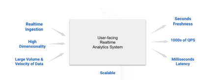 Apache Pinot实时应用程序性能监视Apr 13, 2025 am 11:40 AM
介绍 在当今快节奏的软件开发环境中,确保最佳应用程序性能至关重要。监视实时指标,例如响应时间,错误率和资源利用率可以帮助MAIN
 Chatgpt击中了10亿用户? Openai首席执行官说:'短短几周内翻了一番Apr 13, 2025 am 11:23 AM
“您有几个用户?”他扮演。 阿尔特曼回答说:“我认为我们上次说的是每周5亿个活跃者,而且它正在迅速增长。” “你告诉我,就像在短短几周内翻了一番,”安德森继续说道。 “我说那个私人
 pixtral -12b:Mistral AI&#039;第一个多模型模型 - 分析VidhyaApr 13, 2025 am 11:20 AM
介绍 Mistral发布了其第一个多模式模型,即Pixtral-12b-2409。该模型建立在Mistral的120亿参数Nemo 12B之上。是什么设置了该模型?现在可以拍摄图像和Tex
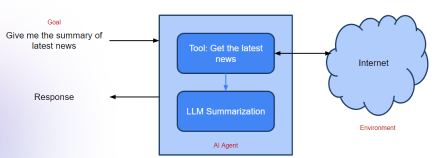 生成AI应用的代理框架 - 分析VidhyaApr 13, 2025 am 11:13 AM
想象一下,拥有一个由AI驱动的助手,不仅可以响应您的查询,还可以自主收集信息,执行任务甚至处理多种类型的数据(TEXT,图像和代码)。听起来有未来派?在这个a


热AI工具

Undresser.AI Undress
人工智能驱动的应用程序,用于创建逼真的裸体照片

AI Clothes Remover
用于从照片中去除衣服的在线人工智能工具。

Undress AI Tool
免费脱衣服图片

Clothoff.io
AI脱衣机

AI Hentai Generator
免费生成ai无尽的。

热门文章
热工具

适用于 Eclipse 的 SAP NetWeaver 服务器适配器
将Eclipse与SAP NetWeaver应用服务器集成。

Atom编辑器mac版下载
最流行的的开源编辑器

ZendStudio 13.5.1 Mac
功能强大的PHP集成开发环境

VSCode Windows 64位 下载
微软推出的免费、功能强大的一款IDE编辑器

禅工作室 13.0.1
功能强大的PHP集成开发环境

