寻找最短路径

两个顶点之间的最短路径是总权重最小的路径。
给定一个边上具有非负权重的图，荷兰计算机科学家 Edsger Dijkstra 发现了一种著名的算法，用于查找两个顶点之间的最短路径。为了找到从顶点 s 到顶点 v 的最短路径，Dijkstra 算法 找到从 s 到所有顶点的最短路径。因此迪杰斯特拉算法被称为单源最短路径算法。该算法使用 cost[v] 来存储从顶点 v 到源顶点 s 的 最短路径 的成本。 成本[s]为0。最初将无穷大分配给所有其他顶点的 cost[v]。该算法重复地在 V – T 中寻找 cost[u] 最小的顶点 u 并将 u 移动到 T .

该算法在下面的代码中描述。

Input: a graph G = (V, E) with non-negative weights
Output: a shortest path tree with the source vertex s as the root
 1 ShortestPathTree getShortestPath(s) {
 2 Let T be a set that contains the vertices whose
 3 paths to s are known; Initially T is empty;
 4 Set cost[s] = 0; and cost[v] = infinity for all other vertices in V;
 5
 6 while (size of T < n) {
 7 Find u not in T with the smallest cost[u];
 8 Add u to T;
 9 for (each v not in T and (u, v) in E)
10 if (cost[v] > cost[u] + w(u, v)) {
11 cost[v] = cost[u] + w(u, v); parent[v] = u;
12 }
13 }
14 }

这个算法与 Prim 寻找最小生成树的算法非常相似。两种算法都将顶点分为两个集合：T 和 V - T。在 Prim 算法的情况下，集合 T 包含已添加到树中的顶点。在 Dijkstra 的情况下，集合 T 包含已找到到源的最短路径的顶点。两种算法都会重复从 V – T 中查找顶点并将其添加到 T。在 Prim 算法的情况下，顶点与集合中边缘权重最小的某个顶点相邻。在 Dijkstra 算法中，该顶点与集合中某个顶点相邻，且对源的总成本最小。

算法首先将 cost[s] 设置为 0（第 4 行），将所有其他顶点的 cost[v] 设置为无穷大。然后，它不断地将一个顶点（比如 u）从 V – T 添加到 T 中，且 cost[u] 最小（第 7 行– 8）、如下图a．将 u 添加到 T 后，算法会更新每个 vcost[v] 和 parent[v] > 不在 T 中，如果 (u, v) 位于 T 且 cost[v] > cost[u] + w(u, v)（第 10-11 行）。

让我们使用下图a中的图来说明Dijkstra算法。假设源顶点是

1。因此，cost[1] = 0 并且所有其他顶点的成本最初为 ∞，如下图 b 所示。我们使用 parent[i] 来表示路径中 i 的父级。为了方便起见，将源节点的父节点设置为 -1.

初始设置

T为空。该算法选择成本最小的顶点。在本例中，顶点为 1。该算法将1添加到T，如下图a所示。然后，它调整与 1 相邻的每个顶点的成本。现在更新了顶点 2、0、6、3 及其父节点的成本，如下图 b.

顶点

2、0、6 和 3 与源顶点相邻，并且顶点 2 是 V-T 中成本最小的一个，因此将 2 添加到 T，如下图所示，并更新顶点的成本和父级V-T 并与 2 相邻。 cost[0] 现已更新为 6，其父级设置为 2。从1到2的箭头线表示将2添加到后，1是2的父级T.

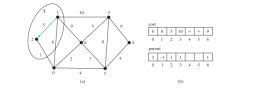
现在 T 包含 {1, 2}。顶点 0 是 V-T 中成本最小的顶点，因此将 0 添加到 T，如下图所示，并更新V-T 中且与 0 相邻的顶点的成本和父级（如果适用）。 cost[5] 现已更新为 10，其父项设置为 0，cost[6] 现已更新为 8 及其父级设置为 0.

现在 T 包含 {1, 2, 0}。顶点 6 是 V-T 中成本最小的顶点，因此将 6 添加到 T，如下图所示，并更新V-T 中且与 6 相邻的顶点的成本和父级（如果适用）。

现在 T 包含 {1, 2, 0, 6}。顶点 3 或 5 是 V-T 中成本最小的一个。您可以将 3 或 5 添加到 T 中。让我们将 3 添加到 T，如下图所示，并更新 V-T 中且与 3 相邻的顶点的成本和父级如果适用。 cost[4] 现已更新为 18，其父级设置为 3。

现在 T 包含 {1, 2, 0, 6, 3}。顶点 5 是 V-T 中成本最小的顶点，因此将 5 添加到 T，如下图所示，并更新V-T 中且与 5 相邻的顶点的成本和父级（如果适用）。 cost[4] 现已更新为 10，其父级设置为 5。

现在 T 包含 {1, 2, 0, 6, 3，5}。顶点 4 是 V-T 中成本最小的顶点，因此将 4 添加到 T，如下图所示。

如您所见，该算法本质上是从源顶点找到所有最短路径，从而生成以源顶点为根的树。我们将此树称为单源全最短路径树（或简称为最短路径树）。要对该树建模，请定义一个名为 ShortestPathTree 的类，该类扩展 Tree 类，如下图所示。 ShortestPathTree 被定义为 WeightedGraph.java 中第 200-224 行 WeightedGraph 中的内部类。

getShortestPath(int sourceVertex) 方法在 WeightedGraph.java 的第 156-197 行中实现。该方法将所有其他顶点的 cost[sourceVertex] 设置为 0 （第 162 行），并将 cost[v] 设置为无穷大（第 159-161 行）。 sourceVertex 的父级设置为 -1（第 166 行）。 T 是一个列表，存储添加到最短路径树中的顶点（第 169 行）。我们使用 T 的列表而不是集合来记录添加到 T 的顶点的顺序。

最初，T 是空的。要展开 T，该方法执行以下操作：

1. Find the vertex u with the smallest cost[u] (lines 175–181) and add it into T (line 183).
2. After adding u in T, update cost[v] and parent[v] for each v adjacent to u in V-T if cost[v] > cost[u] + w(u, v) (lines 186–192).

Once all vertices from s are added to T, an instance of ShortestPathTree is created (line 196).

The ShortestPathTree class extends the Tree class (line 200). To create an instance of ShortestPathTree, pass sourceVertex, parent, T, and cost (lines 204–205). sourceVertex becomes the root in the tree. The data fields root, parent, and searchOrder are defined in the Tree class, which is an inner class defined in AbstractGraph.

Note that testing whether a vertex i is in T by invoking T.contains(i) takes O(n) time, since T is a list. Therefore, the overall time complexity for this implemention is O(n^3).

Dijkstra’s algorithm is a combination of a greedy algorithm and dynamic programming. It is a greedy algorithm in the sense that it always adds a new vertex that has the shortest distance to the source. It stores the shortest distance of each known vertex to the source and uses it later to avoid redundant computing, so Dijkstra’s algorithm also uses dynamic programming.

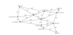
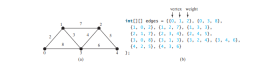
The code below gives a test program that displays the shortest paths from Chicago to all other cities in Figure below and the shortest paths from vertex 3 to all vertices for the graph in Figure below a, respectively.

package demo;

public class TestShortestPath {

    public static void main(String[] args) {
String[] vertices = {"Seattle", "San Francisco", "Los Angeles", "Denver", "Kansas City", "Chicago", "Boston", "New York", "Atlanta", "Miami", "Dallas", "Houston"};

        int[][] edges = {
                {0, 1, 807}, {0, 3, 1331}, {0, 5, 2097},
                {1, 0, 807}, {1, 2, 381}, {1, 3, 1267},
                {2, 1, 381}, {2, 3, 1015}, {2, 4, 1663}, {2, 10, 1435},
                {3, 0, 1331}, {3, 1, 1267}, {3, 2, 1015}, {3, 4, 599}, {3, 5, 1003},
                {4, 2, 1663}, {4, 3, 599}, {4, 5, 533}, {4, 7, 1260}, {4, 8, 864}, {4, 10, 496},
                {5, 0, 2097}, {5, 3, 1003}, {5, 4, 533}, {5, 6, 983}, {5, 7, 787},
                {6, 5, 983}, {6, 7, 214},
                {7, 4, 1260}, {7, 5, 787}, {7, 6, 214}, {7, 8, 888},
                {8, 4, 864}, {8, 7, 888}, {8, 9, 661}, {8, 10, 781}, {8, 11, 810},
                {9, 8, 661}, {9, 11, 1187},
                {10, 2, 1435}, {10, 4, 496}, {10, 8, 781}, {10, 11, 239},
                {11, 8, 810}, {11, 9, 1187}, {11, 10, 239}
        };

        WeightedGraph<String> graph1 = new WeightedGraph<>(vertices, edges);
        WeightedGraph<String>.ShortestPathTree tree1 = graph1.getShortestPath(graph1.getIndex("Chicago"));
        tree1.printAllPaths();

        // Display shortest paths from Houston to Chicago       
        System.out.println("Shortest path from Houston to Chicago: ");
        java.util.List<String> path = tree1.getPath(graph1.getIndex("Houston"));
        for(String s: path) {
            System.out.print(s + " ");
        }

        edges = new int[][]{
            {0, 1, 2}, {0, 3, 8},
            {1, 0, 2}, {1, 2, 7}, {1, 3, 3},
            {2, 1, 7}, {2, 3, 4}, {2, 4, 5},
            {3, 0, 8}, {3, 1, 3}, {3, 2, 4}, {3, 4, 6},
            {4, 2, 5}, {4, 3, 6}
        };

        WeightedGraph<Integer> graph2 = new WeightedGraph<>(edges, 5);
        WeightedGraph<Integer>.ShortestPathTree tree2 = graph2.getShortestPath(3);
        System.out.println("\n");
        tree2.printAllPaths();
    }

}

All shortest paths from Chicago are:
A path from Chicago to Seattle: Chicago Seattle (cost: 2097.0)
A path from Chicago to San Francisco:
Chicago Denver San Francisco (cost: 2270.0)
A path from Chicago to Los Angeles:
Chicago Denver Los Angeles (cost: 2018.0)
A path from Chicago to Denver: Chicago Denver (cost: 1003.0)
A path from Chicago to Kansas City: Chicago Kansas City (cost: 533.0)
A path from Chicago to Chicago: Chicago (cost: 0.0)
A path from Chicago to Boston: Chicago Boston (cost: 983.0)
A path from Chicago to New York: Chicago New York (cost: 787.0)
A path from Chicago to Atlanta:
Chicago Kansas City Atlanta (cost: 1397.0)
A path from Chicago to Miami:
Chicago Kansas City Atlanta Miami (cost: 2058.0)
A path from Chicago to Dallas: Chicago Kansas City Dallas (cost: 1029.0)
A path from Chicago to Houston:
Chicago Kansas City Dallas Houston (cost: 1268.0)
Shortest path from Houston to Chicago:
Houston Dallas Kansas City Chicago

All shortest paths from 3 are:
A path from 3 to 0: 3 1 0 (cost: 5.0)
A path from 3 to 1: 3 1 (cost: 3.0)
A path from 3 to 2: 3 2 (cost: 4.0)
A path from 3 to 3: 3 (cost: 0.0)
A path from 3 to 4: 3 4 (cost: 6.0)

The program creates a weighted graph for Figure above in line 27. It then invokes the getShortestPath(graph1.getIndex("Chicago")) method to return a Path object that contains all shortest paths from Chicago. Invoking printAllPaths() on the ShortestPathTree object displays all the paths (line 30).

The graphical illustration of all shortest paths from Chicago is shown in Figure below. The shortest paths from Chicago to the cities are found in this order: Kansas City, New York, Boston, Denver, Dallas, Houston, Atlanta, Los Angeles, Miami, Seattle, and San Francisco.

以上是寻找最短路径的详细内容。更多信息请关注PHP中文网其他相关文章！