使用Pytorch Geometric 進行連結預測程式碼範例

PyTorch Geometric (PyG)是建構圖神經網路模型和實驗各種圖卷積的主要工具。在本文中我們將透過連結預測來對其進行介紹。

連結預測答了一個問題：哪兩個節點應該相互連結?我們將透過執行“轉換分割”，為建模準備資料。為批次準備專用的圖資料載入器。在Torch Geometric中建立一個模型，使用PyTorch Lightning進行訓練，並檢查模型的表現。

庫準備

• Torch 這個就不用多介紹了
• #Torch Geometric圖形神經網路的主要庫，也是本文介紹的重點
• # PyTorch Lightning 用於訓練、調校和驗證模型。它簡化了訓練的操作
• Sklearn Metrics和Torchmetrics 用於檢查模型的性能。
• PyTorch Geometric有一些特定的依賴關係，如果你安裝有問題，請參閱其官方文件。

資料準備

我們將使用Cora ML引文資料集。資料集可以透過Torch Geometric存取。

 data = tg.datasets.CitationFull(root="data", name="Cora_ML")

預設情況下，Torch Geometric資料集可以傳回多個圖形。我們來看看單一圖是什麼樣子的

data[0] > Data(x=[2995, 2879], edge_index=[2, 16316], y=[2995])

這裡的 X是節點的特徵。 edge_index是2 x (n條邊)矩陣(第一維= 2，被解釋為:第0行-來源節點/“發送方”，第1行-目標節點/“接收方”)。

連結拆分

我們將從拆分資料集中的連結開始。使用20%的圖連結作為驗證集，10%作為測試集。這裡不會向訓練資料集中添加負樣本，因為這樣的負連結將由批次資料載入器即時建立。

一般來說，負採樣會創建「假」樣本(在我們的例子中是節點之間的連結)，因此模型學習如何區分真實和虛假的連結。負抽樣是基於抽樣的理論和數學，具有一些很好的統計性質。

首先:讓我們建立一個連結拆分物件。

 link_splitter = tg.transforms.RandomLinkSplit(num_val=0.2, num_test=0.1, add_negative_train_samples=False,disjoint_train_ratio=0.8)

disjoint_train_ratio調節在「監督」階段將使用多少邊作為訓練資訊。剩餘的邊將用於訊息傳遞(網路中訊息傳遞的階段)。

圖神經網路中至少有兩種分割邊的方法:歸納分割和傳導分割。轉換方法假設GNN需要從圖結構學習結構模式。在歸納設定中，可以使用節點/邊緣標籤進行學習。本文最後有兩篇論文詳細討論了這些概念，並進行了額外的形式化:([1]，[3])。

 train_g, val_g, test_g = link_splitter(data[0])  > Data(x=[2995, 2879], edge_index=[2, 2285], y=[2995], edge_label=[9137], edge_label_index=[2, 9137])

在這個操作之後，我們有了一些新的屬性:

edge_label ：描述邊緣是否為真/假。這是我們想要預測的。

edge_label_index 是一個2 x NUM EDGES矩陣，用於儲存節點連結。

讓我們看看樣本的分佈

th.unique(train_g.edge_label, return_counts=True) > (tensor([1.]), tensor([9137]))  th.unique(val_g.edge_label, return_counts=True) > (tensor([0., 1.]), tensor([3263, 3263]))  th.unique(val_g.edge_label, return_counts=True) > (tensor([0., 1.]), tensor([3263, 3263]))

對於訓練資料沒有負邊(我們將訓練時創建它們)，對於val/測試集——已經以50:50的比例有了一些“假”連結。

模型

現在我們可以在使用GNN進行模型的建構了一個

class GNN(nn.Module):

def __init__(self, dim_in: int, conv_sizes: Tuple[int, ...], act_f: nn.Module = th.relu, dropout: float = 0.1,*args, **kwargs):super().__init__()self.dim_in = dim_inself.dim_out = conv_sizes[-1]self.dropout = dropoutself.act_f = act_flast_in = dim_inlayers = [] # Here we build subsequent graph convolutions.for conv_sz in conv_sizes:# Single graph convolution layerconv = tgnn.SAGEConv(in_channels=last_in, out_channels=conv_sz, *args, **kwargs)last_in = conv_szlayers.append(conv)self.layers = nn.ModuleList(layers) def forward(self, x: th.Tensor, edge_index: th.Tensor) -> th.Tensor:h = x# For every graph convolution in the network...for conv in self.layers:# ... perform node embedding via message passingh = conv(h, edge_index)h = self.act_f(h)if self.dropout:h = nn.functional.dropout(h, p=self.dropout, training=self.training)return h

這個模型中值得注意的部分是一組圖卷積－在我們的例子中是SAGEConv。 SAGE卷積的正式定義為:

å¾ç

v是目前節點，節點v的N(v)個鄰居。要了解更多關於這種卷積類型的信息，請查看GraphSAGE[1]的原始論文

讓我們檢查模型是否可以使用準備好的數據進行預測。這裡PyG模型的輸入是節點特徵X的矩陣和定義edge_index的連結。

gnn = GNN(train_g.x.size()[1], conv_sizes=[512, 256, 128]) with th.no_grad():out = gnn(train_g.x, train_g.edge_index)  out   > tensor([[0.0000, 0.0000, 0.0051, ..., 0.0997, 0.0000, 0.0000],[0.0107, 0.0000, 0.0576, ..., 0.0651, 0.0000, 0.0000],[0.0000, 0.0000, 0.0102, ..., 0.0973, 0.0000, 0.0000],...,[0.0000, 0.0000, 0.0549, ..., 0.0671, 0.0000, 0.0000],[0.0000, 0.0000, 0.0166, ..., 0.0000, 0.0000, 0.0000],[0.0000, 0.0000, 0.0034, ..., 0.1111, 0.0000, 0.0000]])

我們模型的輸出是一個維度為:N個節點x嵌入大小的節點嵌入矩陣。

PyTorch Lightning

PyTorch Lightning主要用作訓練，但是這裡我們在GNN的輸出後面增加了一個Linear層做為預測是否連結的輸出頭。

class LinkPredModel(pl.LightningModule):

def __init__(self,dim_in: int,conv_sizes: Tuple[int, ...], act_f: nn.Module = th.relu, dropout: float = 0.1,lr: float = 0.01,*args, **kwargs):super().__init__() # Our inner GNN modelself.gnn = GNN(dim_in, conv_sizes=conv_sizes, act_f=act_f, dropout=dropout) # Final prediction model on links.self.lin_pred = nn.Linear(self.gnn.dim_out, 1)self.lr = lr def forward(self, x: th.Tensor, edge_index: th.Tensor) -> th.Tensor:# Step 1: make node embeddings using GNN.h = self.gnn(x, edge_index) # Take source nodes embeddings- sendersh_src = h[edge_index[0, :]]# Take target node embeddings - receiversh_dst = h[edge_index[1, :]] # Calculate the product between themsrc_dst_mult = h_src * h_dst# Apply non-linearityout = self.lin_pred(src_dst_mult)return out def _step(self, batch: th.Tensor, phase: str='train') -> th.Tensor:yhat_edge = self(batch.x, batch.edge_label_index).squeeze()y = batch.edge_labelloss = nn.functional.binary_cross_entropy_with_logits(input=yhat_edge, target=y)f1 = tm.functional.f1_score(preds=yhat_edge, target=y, task='binary')prec = tm.functional.precision(preds=yhat_edge, target=y, task='binary')recall = tm.functional.recall(preds=yhat_edge, target=y, task='binary') # Watch for logging here - we need to provide batch_size, as (at the time of this implementation)# PL cannot understand the batch size.self.log(f"{phase}_f1", f1, batch_size=batch.edge_label_index.shape[1])self.log(f"{phase}_loss", loss, batch_size=batch.edge_label_index.shape[1])self.log(f"{phase}_precision", prec, batch_size=batch.edge_label_index.shape[1])self.log(f"{phase}_recall", recall, batch_size=batch.edge_label_index.shape[1])return loss def training_step(self, batch, batch_idx):return self._step(batch) def validation_step(self, batch, batch_idx):return self._step(batch, "val") def test_step(self, batch, batch_idx):return self._step(batch, "test") def predict_step(self, batch):x, edge_index = batchreturn self(x, edge_index) def configure_optimizers(self):return th.optim.Adam(self.parameters(), lr=self.lr)

PyTorch Lightning的作用是幫我們簡化了訓練的步驟，我們只需要配置一些函數即可，我們可以使用以下命令測試模型是否可用

 model = LinkPredModel(val_g.x.size()[1], conv_sizes=[512, 256, 128]) with th.no_grad():out = model.predict_step((val_g.x, val_g.edge_label_index))

訓練

對於訓練的步驟，需要特殊處理的是資料載入器。

圖資料需要特殊處理－尤其是連結預測。 PyG有一些專門的資料載入器類，它們負責正確地產生批次處理。我們將使用:tg.loader.LinkNeighborLoader，它接受以下輸入:

要批次載入的資料(圖)。 num_neighbors 每個節點在一次「跳」期間載入的最大鄰居數量。指定鄰居數目的列表1 - 2 - 3 -…-K。對於非常大的圖形特別有用。

edge_label_index 哪個屬性已經指示了真/假連結。

neg_sampling_ratio -負樣本與真實樣本的比例。

 train_loader = tg.loader.LinkNeighborLoader(train_g,num_neighbors=[-1, 10, 5],batch_size=128,edge_label_index=train_g.edge_label_index, # "on the fly" negative sampling creation for batchneg_sampling_ratio=0.5 )  val_loader = tg.loader.LinkNeighborLoader(val_g,num_neighbors=[-1, 10, 5],batch_size=128,edge_label_index=val_g.edge_label_index,edge_label=val_g.edge_label, # negative samples for val set are done already as ground-truthneg_sampling_ratio=0.0 )  test_loader = tg.loader.LinkNeighborLoader(test_g,num_neighbors=[-1, 10, 5],batch_size=128,edge_label_index=test_g.edge_label_index,edge_label=test_g.edge_label, # negative samples for test set are done already as ground-truthneg_sampling_ratio=0.0 )

以下就是訓練模型

model = LinkPredModel(val_g.x.size()[1], conv_sizes=[512, 256, 128]) trainer = pl.Trainer(max_epochs=20, log_every_n_steps=5)  # Validate before training - we will see results of untrained model. trainer.validate(model, val_loader)  # Train the model trainer.fit(model=model, train_dataloaders=train_loader, val_dataloaders=val_loader)

試驗資料核對，查看分類報告和ROC曲線。

with th.no_grad():yhat_test_proba = th.sigmoid(model(test_g.x, test_g.edge_label_index)).squeeze()yhat_test_cls = yhat_test_proba >= 0.5  print(classification_report(y_true=test_g.edge_label, y_pred=yhat_test_cls))

結果看起來還不錯:

precision recall f1-score support0.0 0.68 0.70 0.69 16311.0 0.69 0.66 0.68 1631accuracy 0.68 3262macro avg 0.68 0.68 0.68 3262

ROC曲线也不错

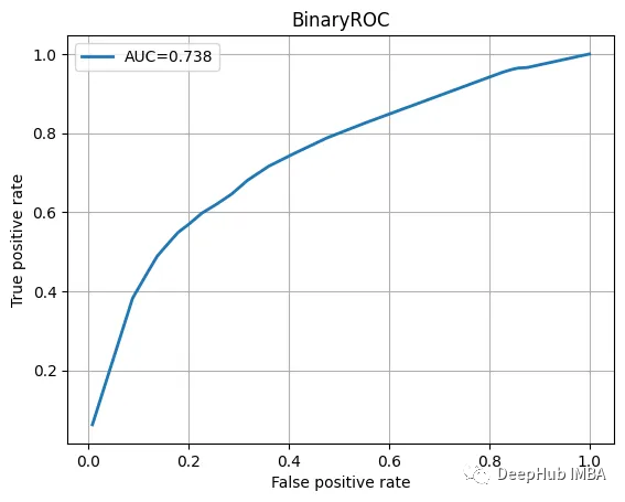
我们训练的模型并不特别复杂，也没有经过精心调整，但它完成了工作。当然这只是一个为了演示使用的小型数据集。

总结

图神经网络尽管看起来很复杂，但是PyTorch Geometric为我们提供了一个很好的解决方案。我们可以直接使用其中内置的模型实现，这方便了我们使用和简化了入门的门槛。

本文代码：https://github.com/maddataanalyst/blogposts_code/blob/main/graph_nns_series/pyg_pyl_perfect_match/pytorch-geometric-lightning-perfect-match.ipynb

以上是使用Pytorch Geometric 進行連結預測程式碼範例的詳細內容。更多資訊請關注PHP中文網其他相關文章！