희소 혼합 전문 아키텍처 언어 모델(MoE)을 처음부터 구현하는 방법을 단계별로 교육합니다.

이 문서에서는 희소 혼합 전문가 언어 모델(MoE)을 구현하는 방법을 소개하고, 희소 혼합 전문가를 사용하여 기존 피드포워드 신경망을 대체하여 Top-K 게이팅을 달성하는 등 모델의 구현 프로세스를 자세히 설명합니다. 및 노이즈 Top-k 게이팅 및 Kaiming He 초기화 기술. 저자는 또한 데이터 세트 처리, 토큰화 전처리 및 언어 모델링 작업과 같이 makemore 아키텍처에서 변경되지 않은 요소를 설명합니다. 마지막으로 모델 구현의 전 과정을 GitHub 저장소 링크로 제공하고 있어 보기 드문 실무 교과서입니다.

소개

혼합 전문가 모델(MoE)은 출시 이후 광범위한 주목을 받기 시작했으며, 특히 희소 혼합 전문가 언어 모델에서 더욱 그렇습니다. 대부분의 구성 요소는 기존 변환기와 유사하지만 상대적으로 단순해 보이지만 희소 혼합 전문가 언어 모델의 훈련 안정성에는 몇 가지 문제가 있습니다.

이 구성 가능한 소규모 희소 MoE 구현 방법은 Hugging Face의 블로그에서 소개되었으며, 이는 새로운 방법을 빠르게 실험하려는 연구자에게 매우 도움이 될 수 있습니다. 또한 블로그에서는 PyTorch를 기반으로 한 자세한 코드를 제공하며 해당 코드는 https://github.com/AviSoori1x/makeMoE/tree/main 링크에서 찾을 수 있습니다. 이러한 소규모 구현은 연구자들이 이 분야에서 신속한 실험을 수행하는 데 도움이 됩니다.

이 웹사이트는 독자의 이익을 위해 이 내용을 편집했습니다.

이 문서에서는 makemore 아키텍처를 기반으로 몇 가지 변경 사항을 적용합니다.

• 별도의 피드포워드 신경망 대신 희소 혼합 전문가 사용

Top-k 게이트 및 노이즈 Top-k 게이팅
매개변수 초기화 Kaiming He 초기화 방법을 사용하지만 이 기사에서는 Xavier/Glorot과 같은 초기화 방법 선택을 포함하여 사용자 정의 가능한 초기화 방법에 중점을 둡니다.
동시에 다음 모듈은 makemore와 일치합니다:

데이터 세트, 전처리(단어 분할) 부분 및 Andrej가 원래 선택한 언어 모델링 작업 - 셰익스피어 스타일로 텍스트 콘텐츠 생성
Casusal Self-Attention 메커니즘
Training loop
Inference logic

실행 계획은 주의 메커니즘부터 시작하여 단계별로 소개됩니다.

Causal Scaled Dot Product Attention Mechanism

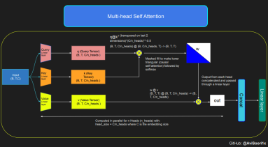다음 코드는 self-attention 메커니즘의 기본 개념을 보여 주며, 고전적인 scaled dot product self-attention을 사용하는 데 중점을 둡니다. self-attention의 이 변형에서는 쿼리 행렬, 키 행렬, 값 행렬이 모두 동일한 입력 시퀀스에서 나옵니다. 동시에, 특히 순수 디코더 모델에서 자동 회귀 언어 생성 프로세스의 무결성을 보장하기 위해 마스킹 메커니즘이 사용됩니다.

이 마스킹 메커니즘은 현재 토큰 위치 이후의 모든 정보를 마스킹하여 모델이 시퀀스의 이전 부분에만 집중하도록 유도할 수 있기 때문에 매우 중요합니다. 토큰 뒤에 있는 콘텐츠를 차단하는 이러한 종류의 주의를 인과적 자기 주의라고 합니다. 희소 혼합 전문가 모델이 디코더 전용 Transformer 아키텍처에만 국한되지 않는다는 점은 주목할 가치가 있습니다. 실제로 이 분야의 많은 중요한 결과는 Transformer 모델의 인코더 및 디코더 구성 요소도 포함하는 T5 아키텍처를 중심으로 이루어졌습니다.

#This code is borrowed from Andrej Karpathy's makemore repository linked in the repo.The self attention layers in Sparse mixture of experts models are the same asin regular transformer modelstorch.manual_seed(1337)B,T,C = 4,8,32 # batch, time, channelsx = torch.randn(B,T,C)# let's see a single Head perform self-attentionhead_size = 16key = nn.Linear(C, head_size, bias=False)query = nn.Linear(C, head_size, bias=False)value = nn.Linear(C, head_size, bias=False)k = key(x) # (B, T, 16)q = query(x) # (B, T, 16)wei =q @ k.transpose(-2, -1) # (B, T, 16) @ (B, 16, T) ---> (B, T, T)tril = torch.tril(torch.ones(T, T))#wei = torch.zeros((T,T))wei = wei.masked_fill(tril == 0, float('-inf'))wei = F.softmax(wei, dim=-1) #B,T,Tv = value(x) #B,T,Hout = wei @ v # (B,T,T) @ (B,T,H) -> (B,T,H)out.shape

torch.Size([4, 8, 16])

그러면 Causal Self-Attention과 Multi-head Causal Self-Attention의 코드는 다음과 같이 정리할 수 있습니다. 다중 헤드 셀프 어텐션은 여러 어텐션 헤드를 병렬로 적용하며, 각 어텐션 헤드는 채널의 일부(임베딩 차원)에만 집중합니다. Multi-head self-attention은 본질적으로 학습 프로세스를 개선하고 고유한 병렬 기능으로 인해 모델 훈련의 효율성을 높입니다. 다음 코드는 과적합을 방지하기 위해 정규화에 드롭아웃을 사용합니다.

#Causal scaled dot product self-Attention Headn_embd = 64n_head = 4n_layer = 4head_size = 16dropout = 0.1class Head(nn.Module):""" one head of self-attention """def __init__(self, head_size):super().__init__()self.key = nn.Linear(n_embd, head_size, bias=False)self.query = nn.Linear(n_embd, head_size, bias=False)self.value = nn.Linear(n_embd, head_size, bias=False)self.register_buffer('tril', torch.tril(torch.ones(block_size, block_size)))self.dropout = nn.Dropout(dropout)def forward(self, x):B,T,C = x.shapek = self.key(x) # (B,T,C)q = self.query(x) # (B,T,C)# compute attention scores ("affinities")wei = q @ k.transpose(-2,-1) * C**-0.5 # (B, T, C) @ (B, C, T) -> (B, T, T)wei = wei.masked_fill(self.tril[:T, :T] == 0, float('-inf')) # (B, T, T)wei = F.softmax(wei, dim=-1) # (B, T, T)wei = self.dropout(wei)# perform the weighted aggregation of the valuesv = self.value(x) # (B,T,C)out = wei @ v # (B, T, T) @ (B, T, C) -> (B, T, C)        return out

Multi-head self-attention의 구현은 다음과 같습니다:

#Multi-Headed Self Attentionclass MultiHeadAttention(nn.Module):""" multiple heads of self-attention in parallel """def __init__(self, num_heads, head_size):super().__init__()self.heads = nn.ModuleList([Head(head_size) for _ in range(num_heads)])self.proj = nn.Linear(n_embd, n_embd)self.dropout = nn.Dropout(dropout)def forward(self, x):out = torch.cat([h(x) for h in self.heads], dim=-1)out = self.dropout(self.proj(out))        return out

전문가 모듈 만들기

즉, 간단한 다층 퍼셉트론

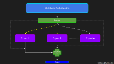
스파스 하이브리드 전문가 아키텍처에서 , 각 변압기 영역 블록 내의 self-attention 메커니즘은 변경되지 않습니다. 그러나 각 블록의 구조는 극적으로 변합니다. 표준 피드포워드

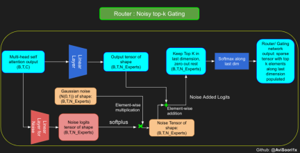
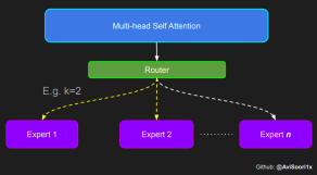
신경망

은 드물게 활성화된 여러 개의 피드포워드 네트워크(예: 전문가 네트워크)로 대체됩니다. 소위 "희소 활성화"는 시퀀스의 각 토큰이 제한된 수의 전문가(보통 한두 명)에게만 할당된다는 것을 의미합니다.

这有助于提高训练和推理速度，因为每次前向传递都会激活少数专家。不过，所有专家都必须存在 GPU 内存中，因此当参数总数达到数千亿甚至数万亿时，就会产生部署方面的问题。

#Expert moduleclass Expert(nn.Module):""" An MLP is a simple linear layer followed by a non-linearity i.e. each Expert """def __init__(self, n_embd):super().__init__()self.net = nn.Sequential(nn.Linear(n_embd, 4 * n_embd),nn.ReLU(),nn.Linear(4 * n_embd, n_embd),nn.Dropout(dropout),)def forward(self, x):        return self.net(x)

Top-k 门控的一个例子

门控网络，也称为路由，确定哪个专家网络接收来自多头注意力的 token 的输出。举个例子解释路由的机制，假设有 4 个专家，token 需要被路由到前 2 个专家中。首先需要通过线性层将 token 输入到门控网络中。该层将对应于（Batch size，Tokens，n_embed）的输入张量从（2，4，32）维度，投影到对应于（Batch size、Tokens，num_expert）的新形状：（2、4，4）。其中 n_embed 是输入的通道维度，num_experts 是专家网络的计数。

接下来，沿最后一个维度，找出最大的前两个值及其相应的索引。

#Understanding how gating worksnum_experts = 4top_k=2n_embed=32#Example multi-head attention output for a simple illustrative example, consider n_embed=32, context_length=4 and batch_size=2mh_output = torch.randn(2, 4, n_embed)topkgate_linear = nn.Linear(n_embed, num_experts) # nn.Linear(32, 4)logits = topkgate_linear(mh_output)top_k_logits, top_k_indices = logits.topk(top_k, dim=-1)# Get top-k expertstop_k_logits, top_k_indices

#output:(tensor([[[ 0.0246, -0.0190],[ 0.1991,0.1513],[ 0.9749,0.7185],[ 0.4406, -0.8357]],  [[ 0.6206, -0.0503],[ 0.8635,0.3784],[ 0.6828,0.5972],[ 0.4743,0.3420]]], grad_fn=<TopkBackward0>), tensor([[[2, 3],[2, 1],[3, 1],[2, 1]],  [[0, 2], [0, 3], [3, 2],         [3, 0]]]))

通过仅保留沿最后一个维度进行比较的前 k 大的值，来获得稀疏门控的输出。用负无穷值填充其余部分，在使用 softmax 激活函数。负无穷会被映射至零，而最大的前两个值会更加突出，且和为 1。要求和为 1 是为了对专家输出的内容进行加权。

zeros = torch.full_like(logits, float('-inf')) #full_like clones a tensor and fills it with a specified value (like infinity) for masking or calculations.sparse_logits = zeros.scatter(-1, top_k_indices, top_k_logits)sparse_logits

#outputtensor([[[ -inf,-inf,0.0246, -0.0190], [ -inf,0.1513,0.1991,-inf], [ -inf,0.7185,-inf,0.9749], [ -inf, -0.8357,0.4406,-inf]],[[ 0.6206,-inf, -0.0503,-inf], [ 0.8635,-inf,-inf,0.3784], [ -inf,-inf,0.5972,0.6828], [ 0.3420,-inf,-inf,0.4743]]], grad_fn=<ScatterBackward0>)

gating_output= F.softmax(sparse_logits, dim=-1)gating_output

#ouputtensor([[[0.0000, 0.0000, 0.5109, 0.4891], [0.0000, 0.4881, 0.5119, 0.0000], [0.0000, 0.4362, 0.0000, 0.5638], [0.0000, 0.2182, 0.7818, 0.0000]],[[0.6617, 0.0000, 0.3383, 0.0000], [0.6190, 0.0000, 0.0000, 0.3810], [0.0000, 0.0000, 0.4786, 0.5214],         [0.4670, 0.0000, 0.0000, 0.5330]]], grad_fn=<SoftmaxBackward0>)

使用有噪声的 top-k 门控以实现负载平衡

# First define the top k router moduleclass TopkRouter(nn.Module):def __init__(self, n_embed, num_experts, top_k):super(TopkRouter, self).__init__()self.top_k = top_kself.linear =nn.Linear(n_embed, num_experts)   def forward(self, mh_ouput):# mh_ouput is the output tensor from multihead self attention blocklogits = self.linear(mh_output)top_k_logits, indices = logits.topk(self.top_k, dim=-1)zeros = torch.full_like(logits, float('-inf'))sparse_logits = zeros.scatter(-1, indices, top_k_logits)router_output = F.softmax(sparse_logits, dim=-1)        return router_output, indices

接下来使用下面这段代码来测试程序：

#Testing this out:num_experts = 4top_k = 2n_embd = 32mh_output = torch.randn(2, 4, n_embd)# Example inputtop_k_gate = TopkRouter(n_embd, num_experts, top_k)gating_output, indices = top_k_gate(mh_output)gating_output.shape, gating_output, indices#And it works!!

#output(torch.Size([2, 4, 4]), tensor([[[0.5284, 0.0000, 0.4716, 0.0000],[0.0000, 0.4592, 0.0000, 0.5408],[0.0000, 0.3529, 0.0000, 0.6471],[0.3948, 0.0000, 0.0000, 0.6052]],  [[0.0000, 0.5950, 0.4050, 0.0000],         [0.4456, 0.0000, 0.5544, 0.0000], [0.7208, 0.0000, 0.0000, 0.2792], [0.0000, 0.0000, 0.5659, 0.4341]]], grad_fn=<SoftmaxBackward0>), tensor([[[0, 2],[3, 1],[3, 1],[3, 0]],  [[1, 2], [2, 0], [0, 3],         [2, 3]]]))

尽管最近发布的 mixtral 的论文没有提到这一点，但本文的作者相信有噪声的 Top-k 门控机制是训练 MoE 模型的一个重要工具。从本质上讲，不会希望所有的 token 都发送给同一组「受欢迎」的专家网络。人们需要的是能在开发和探索之间取得良好平衡。为此，为了负载平衡，从门控的线性层向 logits 激活函数添加标准正态噪声是有帮助的，这使训练更有效率。

#Changing the above to accomodate noisy top-k gatingclass NoisyTopkRouter(nn.Module):def __init__(self, n_embed, num_experts, top_k):super(NoisyTopkRouter, self).__init__()self.top_k = top_k#layer for router logitsself.topkroute_linear = nn.Linear(n_embed, num_experts)self.noise_linear =nn.Linear(n_embed, num_experts)def forward(self, mh_output):# mh_ouput is the output tensor from multihead self attention blocklogits = self.topkroute_linear(mh_output)#Noise logitsnoise_logits = self.noise_linear(mh_output)#Adding scaled unit gaussian noise to the logitsnoise = torch.randn_like(logits)*F.softplus(noise_logits)noisy_logits = logits + noisetop_k_logits, indices = noisy_logits.topk(self.top_k, dim=-1)zeros = torch.full_like(noisy_logits, float('-inf'))sparse_logits = zeros.scatter(-1, indices, top_k_logits)router_output = F.softmax(sparse_logits, dim=-1)        return router_output, indices

再次尝试代码：

#Testing this out, again:num_experts = 8top_k = 2n_embd = 16mh_output = torch.randn(2, 4, n_embd)# Example inputnoisy_top_k_gate = NoisyTopkRouter(n_embd, num_experts, top_k)gating_output, indices = noisy_top_k_gate(mh_output)gating_output.shape, gating_output, indices#It works!!

#output(torch.Size([2, 4, 8]), tensor([[[0.4181, 0.0000, 0.5819, 0.0000, 0.0000, 0.0000, 0.0000, 0.0000],[0.4693, 0.5307, 0.0000, 0.0000, 0.0000, 0.0000, 0.0000, 0.0000],[0.0000, 0.4985, 0.5015, 0.0000, 0.0000, 0.0000, 0.0000, 0.0000],[0.0000, 0.0000, 0.0000, 0.2641, 0.0000, 0.7359, 0.0000, 0.0000]],  [[0.0000, 0.0000, 0.0000, 0.6301, 0.0000, 0.3699, 0.0000, 0.0000], [0.0000, 0.0000, 0.0000, 0.4766, 0.0000, 0.0000, 0.0000, 0.5234], [0.0000, 0.0000, 0.0000, 0.6815, 0.0000, 0.0000, 0.3185, 0.0000], [0.4482, 0.5518, 0.0000, 0.0000, 0.0000, 0.0000, 0.0000, 0.0000]]],        grad_fn=<SoftmaxBackward0>), tensor([[[2, 0],[1, 0],[2, 1],[5, 3]],  [[3, 5], [7, 3], [3, 6],           [1, 0]]]))

创建稀疏化的混合专家模块

在获得门控网络的输出结果之后，对于给定的 token，将前 k 个值选择性地与来自相应的前 k 个专家的输出相乘。这种选择性乘法的结果是一个加权和，该加权和构成 SparseMoe 模块的输出。这个过程的关键和难点是避免不必要的乘法运算，只为前 k 名专家进行正向转播。为每个专家执行前向传播将破坏使用稀疏 MoE 的目的，因为这个过程将不再是稀疏的。

class SparseMoE(nn.Module):def __init__(self, n_embed, num_experts, top_k):super(SparseMoE, self).__init__()self.router = NoisyTopkRouter(n_embed, num_experts, top_k)self.experts = nn.ModuleList([Expert(n_embed) for _ in range(num_experts)])self.top_k = top_kdef forward(self, x):gating_output, indices = self.router(x)final_output = torch.zeros_like(x)# Reshape inputs for batch processingflat_x = x.view(-1, x.size(-1))flat_gating_output = gating_output.view(-1, gating_output.size(-1))# Process each expert in parallelfor i, expert in enumerate(self.experts):# Create a mask for the inputs where the current expert is in top-kexpert_mask = (indices == i).any(dim=-1)flat_mask = expert_mask.view(-1)if flat_mask.any():expert_input = flat_x[flat_mask]expert_output = expert(expert_input)# Extract and apply gating scoresgating_scores = flat_gating_output[flat_mask, i].unsqueeze(1)weighted_output = expert_output * gating_scores# Update final output additively by indexing and addingfinal_output[expert_mask] += weighted_output.squeeze(1)        return final_output

运行以下代码来用样本测试上述实现，可以看到确实如此！

import torchimport torch.nn as nn#Let's test this outnum_experts = 8top_k = 2n_embd = 16dropout=0.1mh_output = torch.randn(4, 8, n_embd)# Example multi-head attention outputsparse_moe = SparseMoE(n_embd, num_experts, top_k)final_output = sparse_moe(mh_output)print("Shape of the final output:", final_output.shape)

Shape of the final output: torch.Size([4, 8, 16])

需要强调的是，如上代码所示，从路由 / 门控网络输出的 top_k 本身也很重要。索引确定了被激活的专家是哪些， 对应的值又决定了权重大小。下图进一步解释了加权求和的概念。

模块整合

将多头自注意力和稀疏混合专家相结合，形成稀疏混合专家 transformer 块。就像在 vanilla transformer 块中一样，也要使用残差以确保训练稳定，并避免梯度消失等问题。此外，要采用层归一化来进一步稳定学习过程。

#Create a self attention + mixture of experts block, that may be repeated several number of timesclass Block(nn.Module):""" Mixture of Experts Transformer block: communication followed by computation (multi-head self attention + SparseMoE) """def __init__(self, n_embed, n_head, num_experts, top_k):# n_embed: embedding dimension, n_head: the number of heads we'd likesuper().__init__()head_size = n_embed // n_headself.sa = MultiHeadAttention(n_head, head_size)self.smoe = SparseMoE(n_embed, num_experts, top_k)self.ln1 = nn.LayerNorm(n_embed)self.ln2 = nn.LayerNorm(n_embed)def forward(self, x):x = x + self.sa(self.ln1(x))x = x + self.smoe(self.ln2(x))        return x

最后，将所有内容整合在一起，形成稀疏混合专家语言模型。

class SparseMoELanguageModel(nn.Module):def __init__(self):super().__init__()# each token directly reads off the logits for the next token from a lookup table      self.token_embedding_table = nn.Embedding(vocab_size, n_embed)        self.position_embedding_table = nn.Embedding(block_size, n_embed)self.blocks = nn.Sequential(*[Block(n_embed, n_head=n_head, num_experts=num_experts,top_k=top_k) for _ in range(n_layer)])self.ln_f = nn.LayerNorm(n_embed) # final layer normself.lm_head = nn.Linear(n_embed, vocab_size)def forward(self, idx, targets=None):B, T = idx.shape# idx and targets are both (B,T) tensor of integerstok_emb = self.token_embedding_table(idx) # (B,T,C)pos_emb = self.position_embedding_table(torch.arange(T, device=device)) # (T,C)x = tok_emb + pos_emb # (B,T,C)x = self.blocks(x) # (B,T,C)x = self.ln_f(x) # (B,T,C)logits = self.lm_head(x) # (B,T,vocab_size)if targets is None:loss = Noneelse:B, T, C = logits.shapelogits = logits.view(B*T, C)targets = targets.view(B*T)loss = F.cross_entropy(logits, targets)return logits, lossdef generate(self, idx, max_new_tokens):# idx is (B, T) array of indices in the current contextfor _ in range(max_new_tokens):# crop idx to the last block_size tokensidx_cond = idx[:, -block_size:]# get the predictionslogits, loss = self(idx_cond)# focus only on the last time steplogits = logits[:, -1, :] # becomes (B, C)# apply softmax to get probabilitiesprobs = F.softmax(logits, dim=-1) # (B, C)# sample from the distributionidx_next = torch.multinomial(probs, num_samples=1) # (B, 1)# append sampled index to the running sequenceidx = torch.cat((idx, idx_next), dim=1) # (B, T+1)        return idx

参数初始化对于深度神经网络的高效训练非常重要。由于专家中存在 ReLU 激活，因此这里使用了 Kaiming He 初始化。也可以尝试在 transformer 中更常用的 Glorot 初始化。杰里米 - 霍华德（Jeremy Howard）的《Fastai》第 2 部分有一个从头开始实现这些功能的精彩讲座：https://course.fast.ai/Lessons/lesson17.html

Glorot 参数初始化通常被用于 transformer 模型，因此这是一个可能提高模型性能的方法。

def kaiming_init_weights(m):if isinstance (m, (nn.Linear)): init.kaiming_normal_(m.weight)model = SparseMoELanguageModel()model.apply(kaiming_init_weights)

本文作者使用 mlflow 跟踪并记录重要指标和训练超参数。

#Using MLFlowm = model.to(device)# print the number of parameters in the modelprint(sum(p.numel() for p in m.parameters())/1e6, 'M parameters')# create a PyTorch optimizeroptimizer = torch.optim.AdamW(model.parameters(), lr=learning_rate)#mlflow.set_experiment("makeMoE")with mlflow.start_run():#If you use mlflow.autolog() this will be automatically logged. I chose to explicitly log here for completenessparams = {"batch_size": batch_size , "block_size" : block_size, "max_iters": max_iters, "eval_interval": eval_interval,"learning_rate": learning_rate, "device": device, "eval_iters": eval_iters, "dropout" : dropout, "num_experts": num_experts, "top_k": top_k }mlflow.log_params(params)for iter in range(max_iters):# every once in a while evaluate the loss on train and val setsif iter % eval_interval == 0 or iter == max_iters - 1:losses = estimate_loss()print(f"step {iter}: train loss {losses['train']:.4f}, val loss {losses['val']:.4f}")metrics = {"train_loss": losses['train'], "val_loss": losses['val']}mlflow.log_metrics(metrics, step=iter)# sample a batch of dataxb, yb = get_batch('train')# evaluate the losslogits, loss = model(xb, yb)optimizer.zero_grad(set_to_none=True)loss.backward()optimizer.step()

8.996545 M parametersstep 0: train loss 5.3223, val loss 5.3166step 100: train loss 2.7351, val loss 2.7429step 200: train loss 2.5125, val loss 2.5233...step 4999: train loss 1.5712, val loss 1.7508

记录训练和验证损失可以很好地指示训练的进展情况。该图显示，可能应该在 4500 次时停止（当验证损失稍微增加时）

接下来可以使用这个模型逐字符自回归地生成文本。

# generate from the model. Not great. Not too bad eithercontext = torch.zeros((1, 1), dtype=torch.long, device=device)print(decode(m.generate(context, max_new_tokens=2000)[0].tolist()))

DUKE VINCENVENTIO:If it ever fecond he town sue kigh now,That thou wold'st is steen 't.SIMNA:Angent her; no, my a born Yorthort,Romeoos soun and lawf to your sawe with ch a woft ttastly defy,To declay the soul art; and meart smad.CORPIOLLANUS:Which I cannot shall do from by born und ot cold warrike,What king we best anone wrave's going of heard and goodThus playvage; you have wold the grace....

本文参考内容：

在实施过程中，作者大量参考了以下出版物：

• 混合专家模型：https://arxiv.org/pdf/2401.04088.pdf

• 超大型神经网络：稀疏门控混合专家层：https://arxiv.org/pdf/1701.06538.pdf

• 来自 Andrej Karpathy 的原始 makemore 实现：https://github.com/karpathy/makemore

还可以尝试以下几种方法，来提高模型性能：

• 提高混合专家模块的效率；

• 尝试不同的神经网络初始化策略；

• 从字符级到子词级的分词；

• 对专家数量和 k 的取值（每个 token 激活的专家数量）进行贝叶斯超参数搜索。这可以归类为神经架构搜索。

• 优化专家能力。

위 내용은 희소 혼합 전문 아키텍처 언어 모델(MoE)을 처음부터 구현하는 방법을 단계별로 교육합니다.의 상세 내용입니다. 자세한 내용은 PHP 중국어 웹사이트의 기타 관련 기사를 참조하세요!