Python을 기반으로 단안 3D 재구성을 구현하는 방법

1. 단안 3차원 재구성 개요

물체 세계의 물체는 3차원이지만, 우리가 얻는 이미지는 2차원이지만, 우리는 이 2차원 이미지로부터 대상의 3차원 정보를 인지할 수 있습니다. 차원적인 이미지. 3차원 재구성 기술은 영상을 일정한 방식으로 처리해 컴퓨터가 인식할 수 있는 3차원 정보를 얻어 대상을 분석하는 기술이다. 단안 3D 재구성은 단일 카메라의 움직임을 기반으로 양안 시력을 시뮬레이션하여 공간에 있는 물체의 3차원 시각 정보를 얻습니다. 단안은 단일 카메라를 의미합니다.

2. 구현 과정

객체의 단안 3D 재구성 과정에서 관련 운영 환경은 다음과 같습니다:

matplotlib 3.3.4
numpy 1.19.5
opencv-contrib-python 3.4.2.16
opencv- python 3.4.2.16
pillow 8.2.0
python 3.6.2

재구성에는 주로 다음 단계가 포함됩니다.

(1) 카메라 보정

(2) 이미지 특징 추출 및 매칭

(3) 3차원 재구성

다음으로 각 단계의 구체적인 구현을 자세히 살펴보겠습니다.

(1) 카메라 보정

휴대폰 카메라, 디지털 카메라, 기능성 모듈 카메라, 등등. 각 카메라의 매개변수는 다릅니다. 즉, 카메라로 촬영한 사진의 해상도, 모드 등이 다릅니다. 물체의 3차원 재구성을 수행할 때 카메라의 매트릭스 매개변수를 미리 모른다고 가정합니다. 그런 다음 카메라의 매트릭스 매개변수를 계산해야 합니다. 이 단계를 카메라 보정이라고 합니다. 카메라 보정의 관련 원리는 소개하지 않겠습니다. 인터넷에서 많은 사람들이 자세히 설명했습니다. 캘리브레이션의 구체적인 구현은 다음과 같습니다.

def camera_calibration(ImagePath):
    # 循环中断
    criteria = (cv2.TERM_CRITERIA_EPS + cv2.TERM_CRITERIA_MAX_ITER, 30, 0.001)
    # 棋盘格尺寸（棋盘格的交叉点的个数）
    row = 11
    column = 8
    
    objpoint = np.zeros((row * column, 3), np.float32)
    objpoint[:, :2] = np.mgrid[0:row, 0:column].T.reshape(-1, 2)

    objpoints = []  # 3d point in real world space
    imgpoints = []  # 2d points in image plane.

    batch_images = glob.glob(ImagePath + '/*.jpg')
    for i, fname in enumerate(batch_images):
        img = cv2.imread(batch_images[i])
        imgGray = cv2.cvtColor(img, cv2.COLOR_BGR2GRAY)
        # find chess board corners
        ret, corners = cv2.findChessboardCorners(imgGray, (row, column), None)
        # if found, add object points, image points (after refining them)
        if ret:
            objpoints.append(objpoint)
            corners2 = cv2.cornerSubPix(imgGray, corners, (11, 11), (-1, -1), criteria)
            imgpoints.append(corners2)
            # Draw and display the corners
            img = cv2.drawChessboardCorners(img, (row, column), corners2, ret)
            cv2.imwrite('Checkerboard_Image/Temp_JPG/Temp_' + str(i) + '.jpg', img)

    print("成功提取:", len(batch_images), "张图片角点！")
    ret, mtx, dist, rvecs, tvecs = cv2.calibrateCamera(objpoints, imgpoints, imgGray.shape[::-1], None, None)

그 중 cv2.calibrateCamera 함수로 얻은 mtx 행렬이 K 행렬입니다.

해당 매개변수를 수정하고 보정을 완료한 후 체커보드의 꼭지점이 성공적으로 추출되었는지 확인하기 위해 체커판의 꼭지점 이미지를 출력할 수 있습니다. 출력된 꼭지점 이미지는 다음과 같습니다.

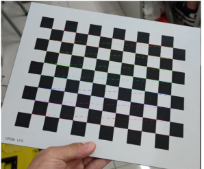
그림 1: 체커보드 모서리 점 추출

(2) 이미지 특징 추출 및 매칭

전체 3차원 재구성 프로세스에서 이 단계는 가장 중요하고 가장 복잡한 단계로 이미지 특징 추출의 품질이 최종 재구성을 결정합니다. 효과.
이미지 특징점 추출 알고리즘 중에는 SIFT 알고리즘, SURF 알고리즘, ORB 알고리즘이라는 세 가지 일반적으로 사용되는 알고리즘이 있습니다. 이 단계에서는 종합적인 분석과 비교를 통해 SURF 알고리즘을 사용하여 이미지의 특징점을 추출합니다. 세 가지 알고리즘의 특징점 추출 효과를 비교하고 싶으시면 온라인으로 검색해 보시고 여기서는 하나씩 비교하지 않겠습니다. 구체적인 구현은 다음과 같습니다.

def epipolar_geometric(Images_Path, K):
    IMG = glob.glob(Images_Path)
    img1, img2 = cv2.imread(IMG[0]), cv2.imread(IMG[1])
    img1_gray = cv2.cvtColor(img1, cv2.COLOR_BGR2GRAY)
    img2_gray = cv2.cvtColor(img2, cv2.COLOR_BGR2GRAY)

    # Initiate SURF detector
    SURF = cv2.xfeatures2d_SURF.create()

    # compute keypoint & descriptions
    keypoint1, descriptor1 = SURF.detectAndCompute(img1_gray, None)
    keypoint2, descriptor2 = SURF.detectAndCompute(img2_gray, None)
    print("角点数量：", len(keypoint1), len(keypoint2))

    # Find point matches
    bf = cv2.BFMatcher(cv2.NORM_L2, crossCheck=True)
    matches = bf.match(descriptor1, descriptor2)
    print("匹配点数量：", len(matches))

    src_pts = np.asarray([keypoint1[m.queryIdx].pt for m in matches])
    dst_pts = np.asarray([keypoint2[m.trainIdx].pt for m in matches])
    # plot
    knn_image = cv2.drawMatches(img1_gray, keypoint1, img2_gray, keypoint2, matches[:-1], None, flags=2)
    image_ = Image.fromarray(np.uint8(knn_image))
    image_.save("MatchesImage.jpg")

    # Constrain matches to fit homography
    retval, mask = cv2.findHomography(src_pts, dst_pts, cv2.RANSAC, 100.0)

    # We select only inlier points
    points1 = src_pts[mask.ravel() == 1]
    points2 = dst_pts[mask.ravel() == 1]

에서 찾은 특징점은 다음과 같습니다.

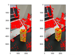
그림 2: 특징점 추출

(3) 3차원 재구성

그림의 특징점을 찾은 후 서로 일치시키면 3차원 재구성을 시작할 수 있습니다. 구체적인 구현은 다음과 같습니다:

points1 = cart2hom(points1.T)
points2 = cart2hom(points2.T)
# plot
fig, ax = plt.subplots(1, 2)
ax[0].autoscale_view('tight')
ax[0].imshow(cv2.cvtColor(img1, cv2.COLOR_BGR2RGB))
ax[0].plot(points1[0], points1[1], 'r.')
ax[1].autoscale_view('tight')
ax[1].imshow(cv2.cvtColor(img2, cv2.COLOR_BGR2RGB))
ax[1].plot(points2[0], points2[1], 'r.')
plt.savefig('MatchesPoints.jpg')
fig.show()
# 

points1n = np.dot(np.linalg.inv(K), points1)
points2n = np.dot(np.linalg.inv(K), points2)
E = compute_essential_normalized(points1n, points2n)
print('Computed essential matrix:', (-E / E[0][1]))

P1 = np.array([[1, 0, 0, 0], [0, 1, 0, 0], [0, 0, 1, 0]])
P2s = compute_P_from_essential(E)

ind = -1
for i, P2 in enumerate(P2s):
    # Find the correct camera parameters
    d1 = reconstruct_one_point(points1n[:, 0], points2n[:, 0], P1, P2)
    # Convert P2 from camera view to world view
    P2_homogenous = np.linalg.inv(np.vstack([P2, [0, 0, 0, 1]]))
    d2 = np.dot(P2_homogenous[:3, :4], d1)
    if d1[2] > 0 and d2[2] > 0:
        ind = i

P2 = np.linalg.inv(np.vstack([P2s[ind], [0, 0, 0, 1]]))[:3, :4]
Points3D = linear_triangulation(points1n, points2n, P1, P2)

fig = plt.figure()
fig.suptitle('3D reconstructed', fontsize=16)
ax = fig.gca(projection='3d')
ax.plot(Points3D[0], Points3D[1], Points3D[2], 'b.')
ax.set_xlabel('x axis')
ax.set_ylabel('y axis')
ax.set_zlabel('z axis')
ax.view_init(elev=135, azim=90)
plt.savefig('Reconstruction.jpg')
plt.show()

재구성 효과는 다음과 같습니다(효과는 평균입니다):

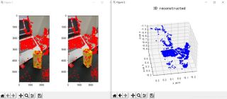
그림 3: 3차원 재구성

III. 결론

재구성 결과에서 단안의 3차원 재구성 효과는 평균적인 것으로 생각됩니다.

(1) 사진 촬영 형식. 단안 3D 재구성 작업을 수행하는 경우 사진을 찍을 때 카메라를 평행하게 계속 움직이는 것이 가장 좋으며 정면에서 사진을 찍는 것이 가장 좋습니다. 즉, 특정 각도나 특정 각도로 사진을 찍지 마십시오.

(2) 사진 촬영 시 주변 환경의 간섭을 받습니다. 관련 없는 물체의 간섭을 줄이려면 단일 촬영 위치를 선택하는 것이 가장 좋습니다.

(3) 촬영 광원 문제. 선택한 사진 위치는 적절한 밝기를 보장해야 하며(광원이 표준을 충족하는지 확인하려면 특정 상황을 테스트해야 함), 카메라를 이동할 때 광원이 이전 순간과 이번 순간 사이에서 일치하는지 확인해야 합니다. 순간.

사실 단안 3D 재구성의 성능은 일반적으로 모든 조건이 최적일 때에도 결과적인 재구성 효과가 그리 좋지 않습니다. 아니면 쌍안 3D 재구성을 사용하는 것을 고려할 수도 있습니다. 단안의 효과보다 확실히 양안 3D 재구성의 효과가 더 좋습니다. 하하. 실제로 작업은 복잡하지 않습니다. 가장 까다로운 부분은 두 카메라를 촬영하고 보정하는 것입니다. 다른 측면은 비교적 쉽습니다.

4.코드

import cv2
import json
import numpy as np
import glob
from PIL import Image
import matplotlib.pyplot as plt
plt.rcParams['font.sans-serif'] = ['SimHei']
plt.rcParams['axes.unicode_minus'] = False


def cart2hom(arr):
    """ Convert catesian to homogenous points by appending a row of 1s
    :param arr: array of shape (num_dimension x num_points)
    :returns: array of shape ((num_dimension+1) x num_points) 
    """
    if arr.ndim == 1:
        return np.hstack([arr, 1])
    return np.asarray(np.vstack([arr, np.ones(arr.shape[1])]))


def compute_P_from_essential(E):
    """ Compute the second camera matrix (assuming P1 = [I 0])
        from an essential matrix. E = [t]R
    :returns: list of 4 possible camera matrices.
    """
    U, S, V = np.linalg.svd(E)

    # Ensure rotation matrix are right-handed with positive determinant
    if np.linalg.det(np.dot(U, V)) < 0:
        V = -V

    # create 4 possible camera matrices (Hartley p 258)
    W = np.array([[0, -1, 0], [1, 0, 0], [0, 0, 1]])
    P2s = [np.vstack((np.dot(U, np.dot(W, V)).T, U[:, 2])).T,
           np.vstack((np.dot(U, np.dot(W, V)).T, -U[:, 2])).T,
           np.vstack((np.dot(U, np.dot(W.T, V)).T, U[:, 2])).T,
           np.vstack((np.dot(U, np.dot(W.T, V)).T, -U[:, 2])).T]

    return P2s


def correspondence_matrix(p1, p2):
    p1x, p1y = p1[:2]
    p2x, p2y = p2[:2]

    return np.array([
        p1x * p2x, p1x * p2y, p1x,
        p1y * p2x, p1y * p2y, p1y,
        p2x, p2y, np.ones(len(p1x))
    ]).T

    return np.array([
        p2x * p1x, p2x * p1y, p2x,
        p2y * p1x, p2y * p1y, p2y,
        p1x, p1y, np.ones(len(p1x))
    ]).T


def scale_and_translate_points(points):
    """ Scale and translate image points so that centroid of the points
        are at the origin and avg distance to the origin is equal to sqrt(2).
    :param points: array of homogenous point (3 x n)
    :returns: array of same input shape and its normalization matrix
    """
    x = points[0]
    y = points[1]
    center = points.mean(axis=1)  # mean of each row
    cx = x - center[0]  # center the points
    cy = y - center[1]
    dist = np.sqrt(np.power(cx, 2) + np.power(cy, 2))
    scale = np.sqrt(2) / dist.mean()
    norm3d = np.array([
        [scale, 0, -scale * center[0]],
        [0, scale, -scale * center[1]],
        [0, 0, 1]
    ])

    return np.dot(norm3d, points), norm3d


def compute_image_to_image_matrix(x1, x2, compute_essential=False):
    """ Compute the fundamental or essential matrix from corresponding points
        (x1, x2 3*n arrays) using the 8 point algorithm.
        Each row in the A matrix below is constructed as
        [x'*x, x'*y, x', y'*x, y'*y, y', x, y, 1]
    """
    A = correspondence_matrix(x1, x2)
    # compute linear least square solution
    U, S, V = np.linalg.svd(A)
    F = V[-1].reshape(3, 3)

    # constrain F. Make rank 2 by zeroing out last singular value
    U, S, V = np.linalg.svd(F)
    S[-1] = 0
    if compute_essential:
        S = [1, 1, 0]  # Force rank 2 and equal eigenvalues
    F = np.dot(U, np.dot(np.diag(S), V))

    return F


def compute_normalized_image_to_image_matrix(p1, p2, compute_essential=False):
    """ Computes the fundamental or essential matrix from corresponding points
        using the normalized 8 point algorithm.
    :input p1, p2: corresponding points with shape 3 x n
    :returns: fundamental or essential matrix with shape 3 x 3
    """
    n = p1.shape[1]
    if p2.shape[1] != n:
        raise ValueError('Number of points do not match.')

    # preprocess image coordinates
    p1n, T1 = scale_and_translate_points(p1)
    p2n, T2 = scale_and_translate_points(p2)

    # compute F or E with the coordinates
    F = compute_image_to_image_matrix(p1n, p2n, compute_essential)

    # reverse preprocessing of coordinates
    # We know that P1' E P2 = 0
    F = np.dot(T1.T, np.dot(F, T2))

    return F / F[2, 2]


def compute_fundamental_normalized(p1, p2):
    return compute_normalized_image_to_image_matrix(p1, p2)


def compute_essential_normalized(p1, p2):
    return compute_normalized_image_to_image_matrix(p1, p2, compute_essential=True)


def skew(x):
    """ Create a skew symmetric matrix *A* from a 3d vector *x*.
        Property: np.cross(A, v) == np.dot(x, v)
    :param x: 3d vector
    :returns: 3 x 3 skew symmetric matrix from *x*
    """
    return np.array([
        [0, -x[2], x[1]],
        [x[2], 0, -x[0]],
        [-x[1], x[0], 0]
    ])


def reconstruct_one_point(pt1, pt2, m1, m2):
    """
        pt1 and m1 * X are parallel and cross product = 0
        pt1 x m1 * X  =  pt2 x m2 * X  =  0
    """
    A = np.vstack([
        np.dot(skew(pt1), m1),
        np.dot(skew(pt2), m2)
    ])
    U, S, V = np.linalg.svd(A)
    P = np.ravel(V[-1, :4])

    return P / P[3]


def linear_triangulation(p1, p2, m1, m2):
    """
    Linear triangulation (Hartley ch 12.2 pg 312) to find the 3D point X
    where p1 = m1 * X and p2 = m2 * X. Solve AX = 0.
    :param p1, p2: 2D points in homo. or catesian coordinates. Shape (3 x n)
    :param m1, m2: Camera matrices associated with p1 and p2. Shape (3 x 4)
    :returns: 4 x n homogenous 3d triangulated points
    """
    num_points = p1.shape[1]
    res = np.ones((4, num_points))

    for i in range(num_points):
        A = np.asarray([
            (p1[0, i] * m1[2, :] - m1[0, :]),
            (p1[1, i] * m1[2, :] - m1[1, :]),
            (p2[0, i] * m2[2, :] - m2[0, :]),
            (p2[1, i] * m2[2, :] - m2[1, :])
        ])

        _, _, V = np.linalg.svd(A)
        X = V[-1, :4]
        res[:, i] = X / X[3]

    return res


def writetofile(dict, path):
    for index, item in enumerate(dict):
        dict[item] = np.array(dict[item])
        dict[item] = dict[item].tolist()
    js = json.dumps(dict)
    with open(path, 'w') as f:
        f.write(js)
        print("参数已成功保存到文件")


def readfromfile(path):
    with open(path, 'r') as f:
        js = f.read()
        mydict = json.loads(js)
    print("参数读取成功")
    return mydict


def camera_calibration(SaveParamPath, ImagePath):
    # 循环中断
    criteria = (cv2.TERM_CRITERIA_EPS + cv2.TERM_CRITERIA_MAX_ITER, 30, 0.001)
    # 棋盘格尺寸
    row = 11
    column = 8
    objpoint = np.zeros((row * column, 3), np.float32)
    objpoint[:, :2] = np.mgrid[0:row, 0:column].T.reshape(-1, 2)

    objpoints = []  # 3d point in real world space
    imgpoints = []  # 2d points in image plane.
    batch_images = glob.glob(ImagePath + '/*.jpg')
    for i, fname in enumerate(batch_images):
        img = cv2.imread(batch_images[i])
        imgGray = cv2.cvtColor(img, cv2.COLOR_BGR2GRAY)
        # find chess board corners
        ret, corners = cv2.findChessboardCorners(imgGray, (row, column), None)
        # if found, add object points, image points (after refining them)
        if ret:
            objpoints.append(objpoint)
            corners2 = cv2.cornerSubPix(imgGray, corners, (11, 11), (-1, -1), criteria)
            imgpoints.append(corners2)
            # Draw and display the corners
            img = cv2.drawChessboardCorners(img, (row, column), corners2, ret)
            cv2.imwrite('Checkerboard_Image/Temp_JPG/Temp_' + str(i) + '.jpg', img)
    print("成功提取:", len(batch_images), "张图片角点！")
    ret, mtx, dist, rvecs, tvecs = cv2.calibrateCamera(objpoints, imgpoints, imgGray.shape[::-1], None, None)
    dict = {'ret': ret, 'mtx': mtx, 'dist': dist, 'rvecs': rvecs, 'tvecs': tvecs}
    writetofile(dict, SaveParamPath)

    meanError = 0
    for i in range(len(objpoints)):
        imgpoints2, _ = cv2.projectPoints(objpoints[i], rvecs[i], tvecs[i], mtx, dist)
        error = cv2.norm(imgpoints[i], imgpoints2, cv2.NORM_L2) / len(imgpoints2)
        meanError += error
    print("total error: ", meanError / len(objpoints))


def epipolar_geometric(Images_Path, K):
    IMG = glob.glob(Images_Path)
    img1, img2 = cv2.imread(IMG[0]), cv2.imread(IMG[1])
    img1_gray = cv2.cvtColor(img1, cv2.COLOR_BGR2GRAY)
    img2_gray = cv2.cvtColor(img2, cv2.COLOR_BGR2GRAY)

    # Initiate SURF detector
    SURF = cv2.xfeatures2d_SURF.create()

    # compute keypoint & descriptions
    keypoint1, descriptor1 = SURF.detectAndCompute(img1_gray, None)
    keypoint2, descriptor2 = SURF.detectAndCompute(img2_gray, None)
    print("角点数量：", len(keypoint1), len(keypoint2))

    # Find point matches
    bf = cv2.BFMatcher(cv2.NORM_L2, crossCheck=True)
    matches = bf.match(descriptor1, descriptor2)
    print("匹配点数量：", len(matches))

    src_pts = np.asarray([keypoint1[m.queryIdx].pt for m in matches])
    dst_pts = np.asarray([keypoint2[m.trainIdx].pt for m in matches])
    # plot
    knn_image = cv2.drawMatches(img1_gray, keypoint1, img2_gray, keypoint2, matches[:-1], None, flags=2)
    image_ = Image.fromarray(np.uint8(knn_image))
    image_.save("MatchesImage.jpg")

    # Constrain matches to fit homography
    retval, mask = cv2.findHomography(src_pts, dst_pts, cv2.RANSAC, 100.0)

    # We select only inlier points
    points1 = src_pts[mask.ravel() == 1]
    points2 = dst_pts[mask.ravel() == 1]

    points1 = cart2hom(points1.T)
    points2 = cart2hom(points2.T)
    # plot
    fig, ax = plt.subplots(1, 2)
    ax[0].autoscale_view('tight')
    ax[0].imshow(cv2.cvtColor(img1, cv2.COLOR_BGR2RGB))
    ax[0].plot(points1[0], points1[1], 'r.')
    ax[1].autoscale_view('tight')
    ax[1].imshow(cv2.cvtColor(img2, cv2.COLOR_BGR2RGB))
    ax[1].plot(points2[0], points2[1], 'r.')
    plt.savefig('MatchesPoints.jpg')
    fig.show()
    # 

    points1n = np.dot(np.linalg.inv(K), points1)
    points2n = np.dot(np.linalg.inv(K), points2)
    E = compute_essential_normalized(points1n, points2n)
    print('Computed essential matrix:', (-E / E[0][1]))

    P1 = np.array([[1, 0, 0, 0], [0, 1, 0, 0], [0, 0, 1, 0]])
    P2s = compute_P_from_essential(E)

    ind = -1
    for i, P2 in enumerate(P2s):
        # Find the correct camera parameters
        d1 = reconstruct_one_point(points1n[:, 0], points2n[:, 0], P1, P2)
        # Convert P2 from camera view to world view
        P2_homogenous = np.linalg.inv(np.vstack([P2, [0, 0, 0, 1]]))
        d2 = np.dot(P2_homogenous[:3, :4], d1)
        if d1[2] > 0 and d2[2] > 0:
            ind = i

    P2 = np.linalg.inv(np.vstack([P2s[ind], [0, 0, 0, 1]]))[:3, :4]
    Points3D = linear_triangulation(points1n, points2n, P1, P2)

    return Points3D


def main():
    CameraParam_Path = 'CameraParam.txt'
    CheckerboardImage_Path = 'Checkerboard_Image'
    Images_Path = 'SubstitutionCalibration_Image/*.jpg'

    # 计算相机参数
    camera_calibration(CameraParam_Path, CheckerboardImage_Path)
    # 读取相机参数
    config = readfromfile(CameraParam_Path)
    K = np.array(config['mtx'])
    # 计算3D点
    Points3D = epipolar_geometric(Images_Path, K)
    # 重建3D点
    fig = plt.figure()
    fig.suptitle('3D reconstructed', fontsize=16)
    ax = fig.gca(projection='3d')
    ax.plot(Points3D[0], Points3D[1], Points3D[2], 'b.')
    ax.set_xlabel('x axis')
    ax.set_ylabel('y axis')
    ax.set_zlabel('z axis')
    ax.view_init(elev=135, azim=90)
    plt.savefig('Reconstruction.jpg')
    plt.show()


if __name__ == '__main__':
    main()

위 내용은 Python을 기반으로 단안 3D 재구성을 구현하는 방법의 상세 내용입니다. 자세한 내용은 PHP 중국어 웹사이트의 기타 관련 기사를 참조하세요!