Python에서 로지스틱 회귀를 해결하기 위해 경사하강법을 구현하는 방법

선형 회귀

1. 선형 회귀 함수의 정의

우도 함수: 결합 표본 값이 주어진 함수

: 어떤 종류의 매개변수 정확히는

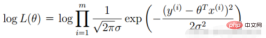
2. 선형 회귀 우도 함수

로그 우도: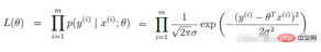

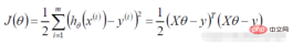
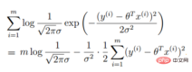3. 선형 회귀 목표 함수

(오류 표현, 우리의 목표는 참값과 예측값 사이의 오차를 최소화하기 위해)

(미분값이 0이 되어 극한값을 구하고, 함수의 모수를 구함)

로지스틱 회귀

로지스틱 회귀를 추가하는 것입니다 선형 회귀 결과에 대한 시그모이드 함수

1. 로지스틱 회귀 함수

2. 로지스틱 회귀 우도 함수

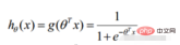데이터가 베르누이 분포를 따른다는 전제

유사한 Ran:

이 경사하강법 작업에

도입되고 로지스틱 회귀 목적 함수

가 경사하강법으로 해결됩니다.

제가 이해한 바는 파생을 통해 매개변수를 업데이트하고 특정 조건에 도달한 후 중지하는 것입니다. , 그리고 대략 최적의 솔루션을 얻습니다.

코드 구현

시그모이드 함수

def sigmoid(z):    
   return 1 / (1 + np.exp(-z))

예측 함수

def model(X, theta):    
    return sigmoid(np.dot(X, theta.T))

목적 함수

def cost(X, y, theta):    
     left = np.multiply(-y, np.log(model(X, theta)))    
     right = np.multiply(1 - y, np.log(1 - model(X, theta)))    
     return np.sum(left - right) / (len(X))

Gradient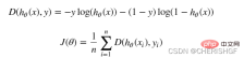

def gradient(X, y, theta):    
  grad = np.zeros(theta.shape)    
  error = (model(X, theta)- y).ravel()    
  for j in range(len(theta.ravel())): #for each parmeter        
     term = np.multiply(error, X[:,j])        
     grad[0, j] = np.sum(term) / len(X)    
   return grad

경사 하강 중지 전략

STOP_ITER = 0
STOP_COST = 1
STOP_GRAD = 2
 
def stopCriterion(type, value, threshold):
    # 设定三种不同的停止策略
    if type == STOP_ITER:  # 设定迭代次数
        return value > threshold
    elif type == STOP_COST:  # 根据损失值停止
        return abs(value[-1] - value[-2]) < threshold
    elif type == STOP_GRAD:  # 根据梯度变化停止
        return np.linalg.norm(value) < threshold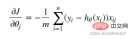

샘플 개편

import numpy.random
#洗牌
def shuffleData(data):
    np.random.shuffle(data)
    cols = data.shape[1]
    X = data[:, 0:cols-1]
    y = data[:, cols-1:]
    return X, y

경사 하강 솔루션

def descent(data, theta, batchSize, stopType, thresh, alpha):
    # 梯度下降求解
 
    init_time = time.time()
    i = 0  # 迭代次数
    k = 0  # batch
    X, y = shuffleData(data)
    grad = np.zeros(theta.shape)  # 计算的梯度
    costs = [cost(X, y, theta)]  # 损失值
 
    while True:
        grad = gradient(X[k:k + batchSize], y[k:k + batchSize], theta)
        k += batchSize  # 取batch数量个数据
        if k >= n:
            k = 0
            X, y = shuffleData(data)  # 重新洗牌
        theta = theta - alpha * grad  # 参数更新
        costs.append(cost(X, y, theta))  # 计算新的损失
        i += 1
 
        if stopType == STOP_ITER:
            value = i
        elif stopType == STOP_COST:
            value = costs
        elif stopType == STOP_GRAD:
            value = grad
        if stopCriterion(stopType, value, thresh): break
 
    return theta, i - 1, costs, grad, time.time() - init_time

전체 코드

import numpy as np
import pandas as pd
import matplotlib.pyplot as plt
import os
import numpy.random
import time
 
 
def sigmoid(z):
    return 1 / (1 + np.exp(-z))
 
 
def model(X, theta):
    return sigmoid(np.dot(X, theta.T))
 
 
def cost(X, y, theta):
    left = np.multiply(-y, np.log(model(X, theta)))
    right = np.multiply(1 - y, np.log(1 - model(X, theta)))
    return np.sum(left - right) / (len(X))
 
 
def gradient(X, y, theta):
    grad = np.zeros(theta.shape)
    error = (model(X, theta) - y).ravel()
    for j in range(len(theta.ravel())):  # for each parmeter
        term = np.multiply(error, X[:, j])
        grad[0, j] = np.sum(term) / len(X)
    return grad
 
 
STOP_ITER = 0
STOP_COST = 1
STOP_GRAD = 2
 
 
def stopCriterion(type, value, threshold):
    # 设定三种不同的停止策略
    if type == STOP_ITER:  # 设定迭代次数
        return value > threshold
    elif type == STOP_COST:  # 根据损失值停止
        return abs(value[-1] - value[-2]) < threshold
    elif type == STOP_GRAD:  # 根据梯度变化停止
        return np.linalg.norm(value) < threshold
 
 
# 洗牌
def shuffleData(data):
    np.random.shuffle(data)
    cols = data.shape[1]
    X = data[:, 0:cols - 1]
    y = data[:, cols - 1:]
    return X, y
 
 
def descent(data, theta, batchSize, stopType, thresh, alpha):
    # 梯度下降求解
 
    init_time = time.time()
    i = 0  # 迭代次数
    k = 0  # batch
    X, y = shuffleData(data)
    grad = np.zeros(theta.shape)  # 计算的梯度
    costs = [cost(X, y, theta)]  # 损失值
 
    while True:
        grad = gradient(X[k:k + batchSize], y[k:k + batchSize], theta)
        k += batchSize  # 取batch数量个数据
        if k >= n:
            k = 0
            X, y = shuffleData(data)  # 重新洗牌
        theta = theta - alpha * grad  # 参数更新
        costs.append(cost(X, y, theta))  # 计算新的损失
        i += 1
 
        if stopType == STOP_ITER:
            value = i
        elif stopType == STOP_COST:
            value = costs
        elif stopType == STOP_GRAD:
            value = grad
        if stopCriterion(stopType, value, thresh): break
 
    return theta, i - 1, costs, grad, time.time() - init_time
 
 
def runExpe(data, theta, batchSize, stopType, thresh, alpha):
    # import pdb
    # pdb.set_trace()
    theta, iter, costs, grad, dur = descent(data, theta, batchSize, stopType, thresh, alpha)
    name = "Original" if (data[:, 1] > 2).sum() > 1 else "Scaled"
    name += " data - learning rate: {} - ".format(alpha)
    if batchSize == n:
        strDescType = "Gradient"  # 批量梯度下降
    elif batchSize == 1:
        strDescType = "Stochastic"  # 随机梯度下降
    else:
        strDescType = "Mini-batch ({})".format(batchSize)  # 小批量梯度下降
    name += strDescType + " descent - Stop: "
    if stopType == STOP_ITER:
        strStop = "{} iterations".format(thresh)
    elif stopType == STOP_COST:
        strStop = "costs change < {}".format(thresh)
    else:
        strStop = "gradient norm < {}".format(thresh)
    name += strStop
    print("***{}\nTheta: {} - Iter: {} - Last cost: {:03.2f} - Duration: {:03.2f}s".format(
        name, theta, iter, costs[-1], dur))
    fig, ax = plt.subplots(figsize=(12, 4))
    ax.plot(np.arange(len(costs)), costs, 'r')
    ax.set_xlabel('Iterations')
    ax.set_ylabel('Cost')
    ax.set_title(name.upper() + ' - Error vs. Iteration')
    return theta
 
 
path = 'data' + os.sep + 'LogiReg_data.txt'
pdData = pd.read_csv(path, header=None, names=['Exam 1', 'Exam 2', 'Admitted'])
positive = pdData[pdData['Admitted'] == 1]
negative = pdData[pdData['Admitted'] == 0]
 
# 画图观察样本情况
fig, ax = plt.subplots(figsize=(10, 5))
ax.scatter(positive['Exam 1'], positive['Exam 2'], s=30, c='b', marker='o', label='Admitted')
ax.scatter(negative['Exam 1'], negative['Exam 2'], s=30, c='r', marker='x', label='Not Admitted')
ax.legend()
ax.set_xlabel('Exam 1 Score')
ax.set_ylabel('Exam 2 Score')
 
pdData.insert(0, 'Ones', 1)
 
# 划分训练数据与标签
orig_data = pdData.values
cols = orig_data.shape[1]
X = orig_data[:, 0:cols - 1]
y = orig_data[:, cols - 1:cols]
# 设置初始参数0
theta = np.zeros([1, 3])
 
# 选择的梯度下降方法是基于所有样本的
n = 100
runExpe(orig_data, theta, n, STOP_ITER, thresh=5000, alpha=0.000001)
runExpe(orig_data, theta, n, STOP_COST, thresh=0.000001, alpha=0.001)
runExpe(orig_data, theta, n, STOP_GRAD, thresh=0.05, alpha=0.001)
runExpe(orig_data, theta, 1, STOP_ITER, thresh=5000, alpha=0.001)
runExpe(orig_data, theta, 1, STOP_ITER, thresh=15000, alpha=0.000002)
runExpe(orig_data, theta, 16, STOP_ITER, thresh=15000, alpha=0.001)
 
from sklearn import preprocessing as pp
 
# 数据预处理
scaled_data = orig_data.copy()
scaled_data[:, 1:3] = pp.scale(orig_data[:, 1:3])
 
runExpe(scaled_data, theta, n, STOP_ITER, thresh=5000, alpha=0.001)
runExpe(scaled_data, theta, n, STOP_GRAD, thresh=0.02, alpha=0.001)
theta = runExpe(scaled_data, theta, 1, STOP_GRAD, thresh=0.002 / 5, alpha=0.001)
runExpe(scaled_data, theta, 16, STOP_GRAD, thresh=0.002 * 2, alpha=0.001)
 
 
# 设定阈值
def predict(X, theta):
    return [1 if x >= 0.5 else 0 for x in model(X, theta)]
 
 
# 计算精度
scaled_X = scaled_data[:, :3]
y = scaled_data[:, 3]
predictions = predict(scaled_X, theta)
correct = [1 if ((a == 1 and b == 1) or (a == 0 and b == 0)) else 0 for (a, b) in zip(predictions, y)]
accuracy = (sum(map(int, correct)) % len(correct))
print('accuracy = {0}%'.format(accuracy))

로지스틱 회귀의 장점과 단점

장점

형태가 간단하고 모델의 해석성이 매우 좋습니다. 특성의 가중치를 통해 다양한 특성이 최종 결과에 미치는 영향을 확인할 수 있습니다. 특정 특성의 가중치 값이 상대적으로 높으면 이 특성이 최종 결과에 더 큰 영향을 미칩니다.

• 모델이 잘 작동하네요. 엔지니어링에서는 (기본적으로) 허용됩니다. 기능 엔지니어링이 잘 수행되면 효과도 나쁘지 않을 것이며 기능 엔지니어링을 병렬로 개발할 수 있어 개발 속도가 크게 향상됩니다.

• 훈련 속도가 빨라졌습니다. 분류할 때 계산량은 특성 수와만 관련됩니다. 또한 로지스틱 회귀의 분산 최적화 sgd는 상대적으로 성숙했으며 힙 머신을 통해 훈련 속도를 더욱 향상시킬 수 있으므로 짧은 시간 내에 여러 버전의 모델을 반복할 수 있습니다.

• 리소스, 특히 메모리를 거의 차지하지 않습니다. 각 차원의 특징값만 저장하면 되기 때문이죠.

• 출력 결과를 조정하는 것이 편리합니다. 로지스틱 회귀는 출력이 각 표본의 확률 점수이기 때문에 쉽게 최종 분류 결과를 얻을 수 있고, 이러한 확률 점수를 쉽게 잘라낼 수 있습니다. 특정 임계값 미만은 하나의 범주로 분류됩니다. 특정 임계값은 범주입니다.

• 단점

정확도가 그다지 높지 않습니다. 형태가 매우 단순하기 때문에(선형 모델과 매우 유사) 데이터의 실제 분포를 맞추기가 어렵습니다.

데이터 불균형 문제를 해결하기가 어렵습니다. 예를 들어, 양성 샘플과 음성 샘플의 비율이 10000:1인 것처럼 양성 샘플과 음성 샘플의 균형이 매우 불균형한 문제를 처리하는 경우 모든 샘플을 양성으로 예측하면 손실 함수의 값을 만들 수도 있습니다. 더 작습니다. 그러나 분류자로서 양성 샘플과 음성 샘플을 구별하는 능력은 그다지 좋지 않습니다.

비선형 데이터를 처리하는 것이 더 까다롭습니다. 로지스틱 회귀는 다른 방법을 도입하지 않고 선형으로 분리 가능한 데이터만 처리하거나 이진 분류 문제를 처리할 수 있습니다.

로지스틱 회귀 자체는 특성을 필터링할 수 없습니다. 때로는 gbdt를 사용하여 기능을 필터링한 다음 로지스틱 회귀를 사용합니다.

위 내용은 Python에서 로지스틱 회귀를 해결하기 위해 경사하강법을 구현하는 방법의 상세 내용입니다. 자세한 내용은 PHP 중국어 웹사이트의 기타 관련 기사를 참조하세요!