
Python을 사용하여 처음부터 필기 회귀 트리

- PHPz앞으로
- 2023-04-14 11:46:021453검색
간단함을 위해 재귀는 트리 노드를 만드는 데 사용됩니다. 비록 재귀가 완벽한 구현은 아니지만 원리를 설명하는 데 가장 직관적입니다.
먼저 라이브러리를 가져옵니다
import pandas as pd
import numpy as np
import matplotlib.pyplot as plt
먼저 훈련 데이터를 만들어야 합니다. 데이터에는 독립 변수(x)와 상관 변수(y)가 있고 numpy를 사용하여 상관 값에 가우스 노이즈를 추가합니다. 수학적으로

여기에 노이즈가 있습니다. 코드는 아래와 같습니다.
def f(x):
mu, sigma = 0, 1.5
return -x**2 + x + 5 + np.random.normal(mu, sigma, 1)
num_points = 300
np.random.seed(1)

x = np.random.uniform(-2, 5, num_points)
y = np.array( [f(i) for i in x] )
plt.scatter(x, y, s = 5)

회귀 트리
회귀 트리에서는 여러 노드로 구성된 트리를 생성하여 수치 데이터를 예측합니다. 아래 그림은 회귀 트리의 트리 구조 예를 보여줍니다. 각 노드에는 데이터를 나누는 데 사용되는 임계값이 있습니다.

데이터 집합이 주어지면 입력 값은 해당 사양을 통해 리프 노드에 도달합니다. 노드 M에 도달하는 모든 입력값은 X의 부분집합으로 표현될 수 있습니다. 수학적으로 이 상황을 주어진 입력 값이 노드 M에 도달하면 1을 주고 그렇지 않으면 0을 주는 함수로 표현해 보겠습니다.

데이터를 분할하는 임계값 찾기: 각 단계에서 2개의 연속 포인트를 선택하고 평균을 계산하여 훈련 데이터를 반복합니다. 계산된 평균은 데이터를 두 개의 임계값으로 나눕니다.
먼저 주어진 상황을 보여주기 위해 임의의 임계값을 고려해 보겠습니다.
threshold = 1.5
low = np.take(y, np.where(x < threshold))
high = np.take(y, np.where(x > threshold))
plt.scatter(x, y, s = 5, label = 'Data')
plt.plot([threshold]*2, [-16, 10], 'b--', label = 'Threshold line')
plt.plot([-2, threshold], [low.mean()]*2, 'r--', label = 'Left child prediction line')
plt.plot([threshold, 5], [high.mean()]*2, 'r--', label = 'Right child prediction line')
plt.plot([-2, 5], [y.mean()]*2, 'g--', label = 'Node prediction line')
plt.legend()

파란색 수직선은 단일 임계값을 나타내며, 이는 두 점의 평균이며 나중에 데이터를 나누는 데 사용된다고 가정합니다.
이 문제에 대한 첫 번째 예측은 모든 훈련 데이터(y축)의 평균(녹색 가로선)입니다. 그리고 두 개의 빨간색 선은 생성될 자식 노드에 대한 예측입니다.
분명히 이러한 평균 중 어느 것도 데이터를 잘 나타내지 않지만 차이점도 분명합니다. 마스터 노드 예측(녹색 선)은 모든 교육 데이터의 평균을 가져오며, 이를 2개의 하위 노드로 나누고 2개의 하위 노드에 자체 노드가 있습니다. 예측(빨간색 선). 녹색 선과 비교할 때 이 두 하위 노드는 해당 훈련 데이터를 더 잘 나타냅니다. 회귀 트리는 데이터를 지속적으로 두 부분으로 분할합니다. 즉, 지정된 중지 값(노드가 가질 수 있는 최소 데이터 양)에 도달할 때까지 각 노드에서 2개의 하위 노드를 생성합니다. 이는 우리가 미리 가지치기한 나무라고 부르는 나무 형성 과정을 조기에 중단합니다.
조기 중지 메커니즘이 있는 이유는 무엇인가요? 노드에 하나의 값만 있을 때까지 계속 할당하면 각 교육 데이터가 자체적으로만 예측할 수 있는 과적합 시나리오가 생성됩니다.
참고: 모델이 완료되면 루트 노드나 중간 노드를 사용하여 값을 예측하지 않고 회귀 트리(트리의 마지막 노드가 됨)의 잎을 사용하여 예측합니다.
주어진 임계값 데이터를 가장 잘 나타내는 임계값을 얻기 위해 잔차 제곱합을 사용합니다. 수학적으로 다음과 같이 정의할 수 있습니다.

이 단계가 어떻게 작동하는지 살펴보겠습니다.

이제 임계값의 SSR 값이 계산되었으므로 최소 SSR 값을 갖는 임계값을 채택할 수 있습니다. 이 임계값을 사용하여 교육 데이터를 두 개(낮은 부분과 높은 부분)로 분할합니다. 여기서 낮은 부분은 왼쪽 자식 노드를 만드는 데 사용되고 높은 부분은 오른쪽 자식 노드를 만드는 데 사용됩니다.
def SSR(r, y):
return np.sum( (r - y)**2 )

SSRs, thresholds = [], []
for i in range(len(x) - 1):
threshold = x[i:i+2].mean()

low = np.take(y, np.where(x < threshold))
high = np.take(y, np.where(x > threshold))

guess_low = low.mean()
guess_high = high.mean()

SSRs.append(SSR(low, guess_low) + SSR(high, guess_high))
thresholds.append(threshold)

print('Minimum residual is: {:.2f}'.format(min(SSRs)))
print('Corresponding threshold value is: {:.4f}'.format(thresholds[SSRs.index(min(SSRs))]))
在进入下一步之前,我将使用pandas创建一个df,并创建一个用于寻找最佳阈值的方法。所有这些步骤都可以在没有pandas的情况下完成,这里使用他是因为比较方便。
df = pd.DataFrame(zip(x, y.squeeze()), columns = ['x', 'y'])
def find_threshold(df, plot = False):
SSRs, thresholds = [], []
for i in range(len(df) - 1):
threshold = df.x[i:i+2].mean()
low = df[(df.x <= threshold)]
high = df[(df.x > threshold)]
guess_low = low.y.mean()
guess_high = high.y.mean()
SSRs.append(SSR(low.y.to_numpy(), guess_low) + SSR(high.y.to_numpy(), guess_high))
thresholds.append(threshold)

if plot:
plt.scatter(thresholds, SSRs, s = 3)
plt.show()

return thresholds[SSRs.index(min(SSRs))]
创建子节点
在将数据分成两个部分后就可以为低值和高值找到单独的阈值。需要注意的是这里要增加一个停止条件;因为对于每个节点,属于该节点的数据集中的点会变少,所以我们为每个节点定义了最小数据点数量。如果不这样做,每个节点将只使用一个训练值进行预测,会导致过拟合。
可以递归地创建节点,我们定义了一个名为TreeNode的类,它将存储节点应该存储的每一个值。使用这个类我们首先创建根,同时计算它的阈值和预测值。然后递归地创建它的子节点,其中每个子节点类都存储在父类的left或right属性中。
在下面的create_nodes方法中,首先将给定的df分成两部分。然后检查是否有足够的数据单独创建左右节点。如果(对于其中任何一个)有足够的数据点,我们计算阈值并使用它创建一个子节点,用这个新节点作为树再次调用create_nodes方法。
class TreeNode():
def __init__(self, threshold, pred):
self.threshold = threshold
self.pred = pred
self.left = None
self.right = None
def create_nodes(tree, df, stop):
low = df[df.x <= tree.threshold]
high = df[df.x > tree.threshold]

if len(low) > stop:
threshold = find_threshold(low)
tree.left = TreeNode(threshold, low.y.mean())
create_nodes(tree.left, low, stop)

if len(high) > stop:
threshold = find_threshold(high)
tree.right = TreeNode(threshold, high.y.mean())
create_nodes(tree.right, high, stop)

threshold = find_threshold(df)
tree = TreeNode(threshold, df.y.mean())
create_nodes(tree, df, 5)
这个方法在第一棵树上进行了修改,因为它不需要返回任何东西。虽然递归函数通常不是这样写的(不返回),但因为不需要返回值,所以当没有激活if语句时,不做任何操作。
在完成后可以检查此树结构,查看它是否创建了一些可以拟合数据的节点。 这里将手动选择第一个节点及其对根阈值的预测。
plt.scatter(x, y, s = 0.5, label = 'Data')
plt.plot([tree.threshold]*2, [-16, 10], 'r--',
label = 'Root threshold')
plt.plot([tree.right.threshold]*2, [-16, 10], 'g--',
label = 'Right node threshold')
plt.plot([tree.threshold, tree.right.threshold],
[tree.right.left.pred]*2,
'g', label = 'Right node prediction')
plt.plot([tree.left.threshold]*2, [-16, 10], 'm--',
label = 'Left node threshold')
plt.plot([tree.left.threshold, tree.threshold],
[tree.left.right.pred]*2,
'm', label = 'Left node prediction')
plt.plot([tree.left.left.threshold]*2, [-16, 10], 'k--',
label = 'Second Left node threshold')
plt.legend()

这里看到了两个预测:
- 第一个左节点对高值的预测(高于其阈值)
- 第一个右节点对低值(低于其阈值)的预测
这里我手动剪切了预测线的宽度,因为如果给定的x值达到了这些节点中的任何一个,则将以属于该节点的所有x值的平均值表示,这也意味着没有其他x值参与 在该节点的预测中(希望有意义)。
这种树形结构远不止两个节点那么简单,所以我们可以通过如下调用它的子节点来检查一个特定的叶子节点。
tree.left.right.left.left
这当然意味着这里有一个向下4个子结点长的分支,但它可以在树的另一个分支上深入得多。
预测
我们可以创建一个预测方法来预测任何给定的值。
def predict(x):
curr_node = tree
result = None
while True:
if x <= curr_node.threshold:
if curr_node.left: curr_node = curr_node.left
else:
break
elif x > curr_node.threshold:
if curr_node.right: curr_node = curr_node.right
else:
break

return curr_node.pred
预测方法做的是沿着树向下,通过比较我们的输入和每个叶子的阈值。如果输入值大于阈值,则转到右叶,如果小于阈值,则转到左叶,以此类推,直到到达任何底部叶子节点。然后使用该节点自身的预测值进行预测,并与其阈值进行最后的比较。
使用x = 3进行测试(在创建数据时,可以使用上面所写的函数计算实际值。-3**2+3+5 = -1,这是期望值),我们得到:
predict(3)
# -1.23741
计算误差
这里用相对平方误差验证数据

def RSE(y, g):
return sum(np.square(y - g)) / sum(np.square(y - 1 / len(y)*sum(y)))
x_val = np.random.uniform(-2, 5, 50)
y_val = np.array( [f(i) for i in x_val] ).squeeze()
tr_preds = np.array( [predict(i) for i in df.x] )
val_preds = np.array( [predict(i) for i in x_val] )
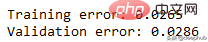
print('Training error: {:.4f}'.format(RSE(df.y, tr_preds)))
print('Validation error: {:.4f}'.format(RSE(y_val, val_preds)))可以看到误差并不大,结果如下

概括的步骤

更深入的模型
一个更适合回归树模型的数据:因为我们的数据是多项式生成的数据,所以使用多项式回归模型可以更好地拟合。我们更换一下训练数据,把新函数设为

def f(x):
mu, sigma = 0, 0.5
if x < 3: return 1 + np.random.normal(mu, sigma, 1)
elif x >= 3 and x < 6: return 9 + np.random.normal(mu, sigma, 1)
elif x >= 6: return 5 + np.random.normal(mu, sigma, 1)

np.random.seed(1)

x = np.random.uniform(0, 10, num_points)
y = np.array( [f(i) for i in x] )
plt.scatter(x, y, s = 5)

在此数据集上运行了上面的所有相同过程,结果如下
比我们从多项式数据中获得的误差低。
最后共享一下上面动图的代码:
import pandas as pd
import numpy as np
import matplotlib.pyplot as plt
from matplotlib.animation import FuncAnimation
#===================================================Create Data
def f(x):
mu, sigma = 0, 1.5
return -x**2 + x + 5 + np.random.normal(mu, sigma, 1)
np.random.seed(1)

x = np.random.uniform(-2, 5, 300)
y = np.array( [f(i) for i in x] )
p = x.argsort()
x = x[p]
y = y[p]
#===================================================Calculate Thresholds
def SSR(r, y): #send numpy array
return np.sum( (r - y)**2 )
SSRs, thresholds = [], []
for i in range(len(x) - 1):
threshold = x[i:i+2].mean()

low = np.take(y, np.where(x < threshold))
high = np.take(y, np.where(x > threshold))

guess_low = low.mean()
guess_high = high.mean()

SSRs.append(SSR(low, guess_low) + SSR(high, guess_high))
thresholds.append(threshold)
#===================================================Animated Plot
fig, (ax1, ax2) = plt.subplots(2,1, sharex = True)
x_data, y_data = [], []
x_data2, y_data2 = [], []
ln, = ax1.plot([], [], 'r--')
ln2, = ax2.plot(thresholds, SSRs, 'ro', markersize = 2)
line = [ln, ln2]
def init():
ax1.scatter(x, y, s = 3)
ax1.title.set_text('Trying Different Thresholds')
ax2.title.set_text('Threshold vs SSR')
ax1.set_ylabel('y values')
ax2.set_xlabel('Threshold')
ax2.set_ylabel('SSR')
return line
def update(frame):
x_data = [x[frame:frame+2].mean()] * 2
y_data = [min(y), max(y)]
line[0].set_data(x_data, y_data)
x_data2.append(thresholds[frame])
y_data2.append(SSRs[frame])
line[1].set_data(x_data2, y_data2)
return line
ani = FuncAnimation(fig, update, frames = 298,
init_func = init, blit = True)
plt.show()
위 내용은 Python을 사용하여 처음부터 필기 회귀 트리의 상세 내용입니다. 자세한 내용은 PHP 중국어 웹사이트의 기타 관련 기사를 참조하세요!