Python으로 3차원 그래프를 그리는 방법에 대한 자세한 튜토리얼

이 기사에서는 Python에 대한 관련 지식을 제공합니다. 일반적으로 우리는 2차원 평면 다이어그램을 그릴 때 Python을 사용하지만 때로는 3차원 장면 다이어그램을 그려야 할 때도 있습니다. 다음은 3차원 드로잉을 위한 Python 관련 정보를 소개합니다. 다이어그램이 모두에게 도움이 되기를 바랍니다.

【관련 추천: Python3 동영상 튜토리얼】

이 글은 가장 기본적인 그리기 방법만을 요약한 것입니다.

1. 초기화

matplotlib 도구 패키지가 설치된 것으로 가정합니다.

matplotlib.Figure.Figure를 사용하여 프레임 만들기:

import matplotlib.pyplot as plt
from mpl_toolkits.mplot3d import Axes3D
fig = plt.figure()
ax = fig.add_subplot(111, projection='3d')

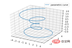
2. 선 플롯

기본 사용법:

ax.plot(x,y,z,label=' ')

코드:

import matplotlib as mpl
from mpl_toolkits.mplot3d import Axes3D
import numpy as np
import matplotlib.pyplot as plt
 
mpl.rcParams['legend.fontsize'] = 10
 
fig = plt.figure()
ax = fig.gca(projection='3d')
theta = np.linspace(-4 * np.pi, 4 * np.pi, 100)
z = np.linspace(-2, 2, 100)
r = z**2 + 1
x = r * np.sin(theta)
y = r * np.cos(theta)
ax.plot(x, y, z, label='parametric curve')
ax.legend()
 
plt.show()

3. 산점도 플롯)

기본 사용법:

ax.scatter(xs, ys, zs, s=20, c=None, depthshade=True, *args, *kwargs)

• xs,ys,zs: 입력 데이터
• s: 산점의 크기
• c: 색상, 예: c = 'r'은 빨간색입니다.
• lengthshase: 투명도, True는 투명합니다. True, False는 불투명합니다.
• *args 등은 확장 변수입니다(예:maker = 'o'). 그러면 분산 결과는 'o' 모양입니다.

code:

from mpl_toolkits.mplot3d import Axes3D
import matplotlib.pyplot as plt
import numpy as np
 
 
def randrange(n, vmin, vmax):
    '''
    Helper function to make an array of random numbers having shape (n, )
    with each number distributed Uniform(vmin, vmax).
    '''
    return (vmax - vmin)*np.random.rand(n) + vmin
 
fig = plt.figure()
ax = fig.add_subplot(111, projection='3d')
 
n = 100
 
# For each set of style and range settings, plot n random points in the box
# defined by x in [23, 32], y in [0, 100], z in [zlow, zhigh].
for c, m, zlow, zhigh in [('r', 'o', -50, -25), ('b', '^', -30, -5)]:
    xs = randrange(n, 23, 32)
    ys = randrange(n, 0, 100)
    zs = randrange(n, zlow, zhigh)
    ax.scatter(xs, ys, zs, c=c, marker=m)
 
ax.set_xlabel('X Label')
ax.set_ylabel('Y Label')
ax.set_zlabel('Z Label')
 
plt.show()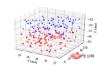

4. 라인 블록 다이어그램(와이어프레임 플롯)

기본 사용법:

ax.plot_wireframe(X, Y, Z, *args, **kwargs)

• X, Y, Z: 입력 데이터
• rstride: 행 단계 길이
• cstride: 열 단계 길이
• rcount: 행 번호의 상한
• ccount: 상한 열 수 제한

code:

from mpl_toolkits.mplot3d import axes3d
import matplotlib.pyplot as plt
 
 
fig = plt.figure()
ax = fig.add_subplot(111, projection='3d')
 
# Grab some test data.
X, Y, Z = axes3d.get_test_data(0.05)
 
# Plot a basic wireframe.
ax.plot_wireframe(X, Y, Z, rstride=10, cstride=10)
 
plt.show()

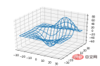
5. 표면 플롯

기본 사용법:

ax.plot_surface(X, Y, Z, *args, **kwargs)

color: 표면 색상
• cmap: 레이어
• code:

6 . 삼중 표면 플롯

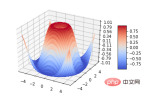기본 사용법:

from mpl_toolkits.mplot3d import Axes3D
import matplotlib.pyplot as plt
from matplotlib import cm
from matplotlib.ticker import LinearLocator, FormatStrFormatter
import numpy as np
 
 
fig = plt.figure()
ax = fig.gca(projection='3d')
 
# Make data.
X = np.arange(-5, 5, 0.25)
Y = np.arange(-5, 5, 0.25)
X, Y = np.meshgrid(X, Y)
R = np.sqrt(X**2 + Y**2)
Z = np.sin(R)
 
# Plot the surface.
surf = ax.plot_surface(X, Y, Z, cmap=cm.coolwarm,
                       linewidth=0, antialiased=False)
 
# Customize the z axis.
ax.set_zlim(-1.01, 1.01)
ax.zaxis.set_major_locator(LinearLocator(10))
ax.zaxis.set_major_formatter(FormatStrFormatter('%.02f'))
 
# Add a color bar which maps values to colors.
fig.colorbar(surf, shrink=0.5, aspect=5)
 
plt.show()

X, Y, Z: 데이터

다른 매개변수는 표면 플롯과 유사합니다

• 코드:

• ax.plot_trisurf(*args, **kwargs)

7. 등고선 플롯

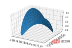기본 사용법 :

from mpl_toolkits.mplot3d import Axes3D
import matplotlib.pyplot as plt
import numpy as np
 
 
n_radii = 8
n_angles = 36
 
# Make radii and angles spaces (radius r=0 omitted to eliminate duplication).
radii = np.linspace(0.125, 1.0, n_radii)
angles = np.linspace(0, 2*np.pi, n_angles, endpoint=False)
 
# Repeat all angles for each radius.
angles = np.repeat(angles[..., np.newaxis], n_radii, axis=1)
 
# Convert polar (radii, angles) coords to cartesian (x, y) coords.
# (0, 0) is manually added at this stage,  so there will be no duplicate
# points in the (x, y) plane.
x = np.append(0, (radii*np.cos(angles)).flatten())
y = np.append(0, (radii*np.sin(angles)).flatten())
 
# Compute z to make the pringle surface.
z = np.sin(-x*y)
 
fig = plt.figure()
ax = fig.gca(projection='3d')
 
ax.plot_trisurf(x, y, z, linewidth=0.2, antialiased=True)
 
plt.show()

code:

ax.contour(X, Y, Z, *args, **kwargs)

2차원 윤곽선, 3차원 표면 지도로 그릴 수도 있습니다:

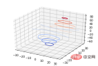code:

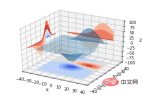
from mpl_toolkits.mplot3d import axes3d
import matplotlib.pyplot as plt
from matplotlib import cm
 
fig = plt.figure()
ax = fig.add_subplot(111, projection='3d')
X, Y, Z = axes3d.get_test_data(0.05)
cset = ax.contour(X, Y, Z, cmap=cm.coolwarm)
ax.clabel(cset, fontsize=9, inline=1)
 
plt.show()

3차원 투영일 수도 있습니다 2차원 평면의 윤곽:

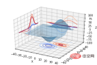코드:

from mpl_toolkits.mplot3d import axes3d
from mpl_toolkits.mplot3d import axes3d
import matplotlib.pyplot as plt
from matplotlib import cm
 
fig = plt.figure()
ax = fig.gca(projection='3d')
X, Y, Z = axes3d.get_test_data(0.05)
ax.plot_surface(X, Y, Z, rstride=8, cstride=8, alpha=0.3)
cset = ax.contour(X, Y, Z, zdir='z', offset=-100, cmap=cm.coolwarm)
cset = ax.contour(X, Y, Z, zdir='x', offset=-40, cmap=cm.coolwarm)
cset = ax.contour(X, Y, Z, zdir='y', offset=40, cmap=cm.coolwarm)
 
ax.set_xlabel('X')
ax.set_xlim(-40, 40)
ax.set_ylabel('Y')
ax.set_ylim(-40, 40)
ax.set_zlabel('Z')
ax.set_zlim(-100, 100)
 
plt.show()

8. 막대 그래프 그림)

기본 사용법:

from mpl_toolkits.mplot3d import axes3d
import matplotlib.pyplot as plt
from matplotlib import cm
 
fig = plt.figure()
ax = fig.gca(projection='3d')
X, Y, Z = axes3d.get_test_data(0.05)
ax.plot_surface(X, Y, Z, rstride=8, cstride=8, alpha=0.3)
cset = ax.contourf(X, Y, Z, zdir='z', offset=-100, cmap=cm.coolwarm)
cset = ax.contourf(X, Y, Z, zdir='x', offset=-40, cmap=cm.coolwarm)
cset = ax.contourf(X, Y, Z, zdir='y', offset=40, cmap=cm.coolwarm)
 
ax.set_xlabel('X')
ax.set_xlim(-40, 40)
ax.set_ylabel('Y')
ax.set_ylim(-40, 40)
ax.set_zlabel('Z')
ax.set_zlim(-100, 100)
 
plt.show()

x, y, zs = z, 데이터

zdir: 막대의 방향 코드에 따라 자세히 이해할 수 있는 막대 차트 평탄화.

• 코드:

• ax.bar(left, height, zs=0, zdir='z', *args, **kwargs

9. 서브플롯(subplot)

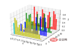3차원 공간에 분산된 색다른 2차원 그래픽, 사실 투영 공간은 비어 있지 않습니다. 해당 코드:

from mpl_toolkits.mplot3d import Axes3D
import matplotlib.pyplot as plt
import numpy as np
 
fig = plt.figure()
ax = fig.add_subplot(111, projection='3d')
for c, z in zip(['r', 'g', 'b', 'y'], [30, 20, 10, 0]):
    xs = np.arange(20)
    ys = np.random.rand(20)
 
    # You can provide either a single color or an array. To demonstrate this,
    # the first bar of each set will be colored cyan.
    cs = [c] * len(xs)
    cs[0] = 'c'
    ax.bar(xs, ys, zs=z, zdir='y', color=cs, alpha=0.8)
 
ax.set_xlabel('X')
ax.set_ylabel('Y')
ax.set_zlabel('Z')
 
plt.show()

B-서브플롯 사용법

MATLAB과의 차이점은 4-서브플롯 효과가 다음과 같다는 것입니다.

보충제:

텍스트 댓글의 기본 사용법:

코드:

from mpl_toolkits.mplot3d import Axes3D
import numpy as np
import matplotlib.pyplot as plt
 
fig = plt.figure()
ax = fig.gca(projection='3d')
 
# Plot a sin curve using the x and y axes.
x = np.linspace(0, 1, 100)
y = np.sin(x * 2 * np.pi) / 2 + 0.5
ax.plot(x, y, zs=0, zdir='z', label='curve in (x,y)')
 
# Plot scatterplot data (20 2D points per colour) on the x and z axes.
colors = ('r', 'g', 'b', 'k')
x = np.random.sample(20*len(colors))
y = np.random.sample(20*len(colors))
c_list = []
for c in colors:
    c_list.append([c]*20)
# By using zdir='y', the y value of these points is fixed to the zs value 0
# and the (x,y) points are plotted on the x and z axes.
ax.scatter(x, y, zs=0, zdir='y', c=c_list, label='points in (x,z)')
 
# Make legend, set axes limits and labels
ax.legend()
ax.set_xlim(0, 1)
ax.set_ylim(0, 1)
ax.set_zlim(0, 1)
ax.set_xlabel('X')
ax.set_ylabel('Y')
ax.set_zlabel('Z')

[관련 권장 사항:

Python3 비디오 튜토리얼

]

위 내용은 Python으로 3차원 그래프를 그리는 방법에 대한 자세한 튜토리얼의 상세 내용입니다. 자세한 내용은 PHP 중국어 웹사이트의 기타 관련 기사를 참조하세요!