비정상적인 데이터를 제거하는 네 가지 방법은 무엇입니까?

비정상 데이터를 제거하는 네 가지 방법은 다음과 같습니다. 1. "격리 포리스트", 2. DBSCAN, 3. OneClassSVM, 4. 샘플의 비정상성을 반영하기 위해 수치 점수를 계산합니다.

이 튜토리얼의 운영 환경: Windows 7 시스템, Dell G3 컴퓨터.

이상치 검출 이상점 식별 방법

1. 격리 숲 격리 숲

1.1 테스트 샘플 예

파일 test.pkl

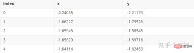
1.2 격리 숲 데모

격리 숲 원리

를 무작위로 나누어 설정 랜덤 포레스트로 하고, 소수의 분할 후에 나누어질 수 있는 점을 비정상 점으로 간주한다.

# 参考https://blog.csdn.net/ye1215172385/article/details/79762317 
# 官方例子https://scikit-learn.org/stable/auto_examples/ensemble/plot_isolation_forest.html#sphx-glr-auto-examples-ensemble-plot-isolation-forest-py
import numpy as np
import matplotlib.pyplot as plt
from sklearn.ensemble import IsolationForest
 
rng = np.random.RandomState(42)
 
# 构造训练样本
n_samples = 200  #样本总数
outliers_fraction = 0.25  #异常样本比例
n_inliers = int((1. - outliers_fraction) * n_samples)
n_outliers = int(outliers_fraction * n_samples)
 
X = 0.3 * rng.randn(n_inliers // 2, 2)
X_train = np.r_[X + 2, X - 2]   #正常样本
X_train = np.r_[X_train, np.random.uniform(low=-6, high=6, size=(n_outliers, 2))]  #正常样本加上异常样本
 
# 构造模型并拟合
clf = IsolationForest(max_samples=n_samples, random_state=rng, contamination=outliers_fraction)
clf.fit(X_train)
# 计算得分并设置阈值
scores_pred = clf.decision_function(X_train)
threshold = np.percentile(scores_pred, 100 * outliers_fraction)  #根据训练样本中异常样本比例，得到阈值，用于绘图
 
# plot the line, the samples, and the nearest vectors to the plane
xx, yy = np.meshgrid(np.linspace(-7, 7, 50), np.linspace(-7, 7, 50))
Z = clf.decision_function(np.c_[xx.ravel(), yy.ravel()])
Z = Z.reshape(xx.shape)
 
plt.title("IsolationForest")
# plt.contourf(xx, yy, Z, cmap=plt.cm.Blues_r)
plt.contourf(xx, yy, Z, levels=np.linspace(Z.min(), threshold, 7), cmap=plt.cm.Blues_r)  #绘制异常点区域，值从最小的到阈值的那部分
a = plt.contour(xx, yy, Z, levels=[threshold], linewidths=2, colors='red')  #绘制异常点区域和正常点区域的边界
plt.contourf(xx, yy, Z, levels=[threshold, Z.max()], colors='palevioletred')  #绘制正常点区域，值从阈值到最大的那部分
 
b = plt.scatter(X_train[:-n_outliers, 0], X_train[:-n_outliers, 1], c='white',
                    s=20, edgecolor='k')
c = plt.scatter(X_train[-n_outliers:, 0], X_train[-n_outliers:, 1], c='black',
                    s=20, edgecolor='k')
plt.axis('tight')
plt.xlim((-7, 7))
plt.ylim((-7, 7))
plt.legend([a.collections[0], b, c],
           ['learned decision function', 'true inliers', 'true outliers'],
           loc="upper left")
plt.show()

1.3 직접 수정하면 X_train을 필요한 데이터로 변경할 수 있습니다.

여기에는 표준화가 없습니다. 먼저 표준화한 다음 sklearn.preprocessing import StandardScaler

import numpy as np
import matplotlib.pyplot as plt
from sklearn.ensemble import IsolationForest
from scipy import stats
 
rng = np.random.RandomState(42)
 
 
X_train =  X_train_demo.values
outliers_fraction = 0.1
n_samples = 500
# 构造模型并拟合
clf = IsolationForest(max_samples=n_samples, random_state=rng, contamination=outliers_fraction)
clf.fit(X_train)
# 计算得分并设置阈值
scores_pred = clf.decision_function(X_train)
threshold = stats.scoreatpercentile(scores_pred, 100 * outliers_fraction)  #根据训练样本中异常样本比例，得到阈值，用于绘图
 
# plot the line, the samples, and the nearest vectors to the plane
range_max_min0 = (X_train[:,0].max()-X_train[:,0].min())*0.2
range_max_min1 = (X_train[:,1].max()-X_train[:,1].min())*0.2
xx, yy = np.meshgrid(np.linspace(X_train[:,0].min()-range_max_min0, X_train[:,0].max()+range_max_min0, 500),
                     np.linspace(X_train[:,1].min()-range_max_min1, X_train[:,1].max()+range_max_min1, 500))
Z = clf.decision_function(np.c_[xx.ravel(), yy.ravel()])
Z = Z.reshape(xx.shape)
 
plt.title("IsolationForest")
# plt.contourf(xx, yy, Z, cmap=plt.cm.Blues_r)
plt.contourf(xx, yy, Z, levels=np.linspace(Z.min(), threshold, 7), cmap=plt.cm.Blues_r)  #绘制异常点区域，值从最小的到阈值的那部分
a = plt.contour(xx, yy, Z, levels=[threshold], linewidths=2, colors='red')  #绘制异常点区域和正常点区域的边界
plt.contourf(xx, yy, Z, levels=[threshold, Z.max()], colors='palevioletred')  #绘制正常点区域，值从阈值到最大的那部分
 
 
is_in = clf.predict(X_train)>0
b = plt.scatter(X_train[is_in, 0], X_train[is_in, 1], c='white',
                    s=20, edgecolor='k')
c = plt.scatter(X_train[~is_in, 0], X_train[~is_in, 1], c='black',
                    s=20, edgecolor='k')
plt.axis('tight')
plt.xlim((X_train[:,0].min()-range_max_min0, X_train[:,0].max()+range_max_min0,))
plt.ylim((X_train[:,1].min()-range_max_min1, X_train[:,1].max()+range_max_min1,))
plt.legend([a.collections[0], b, c],
           ['learned decision function', 'inliers', 'outliers'],
           loc="upper left")
plt.show()

1.4 핵심 코드에서 표준화를 기반으로 이상값을 제거할 수 있습니다.

1.4.1 샘플 샘플

import numpy as np
# 构造训练样本
n_samples = 200  #样本总数
outliers_fraction = 0.25  #异常样本比例
n_inliers = int((1. - outliers_fraction) * n_samples)
n_outliers = int(outliers_fraction * n_samples)
 
X = 0.3 * rng.randn(n_inliers // 2, 2)
X_train = np.r_[X + 2, X - 2]   #正常样本
X_train = np.r_[X_train, np.random.uniform(low=-6, high=6, size=(n_outliers, 2))]  #正常样本加上异常样本

1.4.2 핵심 코드 구현

clf = IsolationForest(max_samples=0.8, 오염=0.25)

from sklearn.ensemble import IsolationForest
# fit the model
# max_samples 构造一棵树使用的样本数，输入大于1的整数则使用该数字作为构造的最大样本数目，
# 如果数字属于(0,1]则使用该比例的数字作为构造iforest
# outliers_fraction 多少比例的样本可以作为异常值
clf = IsolationForest(max_samples=0.8, contamination=0.25)
clf.fit(X_train)
# y_pred_train = clf.predict(X_train)
scores_pred = clf.decision_function(X_train)
threshold = np.percentile(scores_pred, 100 * outliers_fraction)  #根据训练样本中异常样本比例，得到阈值，用于绘图

## 以下两种方法的筛选结果，完全相同
X_train_predict1 = X_train[clf.predict(X_train)==1]
X_train_predict2 = X_train[scores_pred>=threshold,:]
# 其中，1的表示非异常点，-1的表示为异常点
clf.predict(X_train)
array([ 1,  1,  1,  1,  1,  1,  1,  1,  1,  1,  1,  1,  1,  1,  1,  1,  1,
        1,  1,  1,  1,  1,  1,  1,  1,  1,  1,  1,  1,  1,  1,  1,  1,  1,
        1,  1,  1,  1,  1,  1,  1,  1,  1,  1,  1,  1,  1,  1,  1,  1,  1,
        1,  1,  1,  1,  1,  1,  1,  1,  1,  1,  1,  1,  1,  1,  1,  1, -1,
        1,  1,  1,  1,  1,  1,  1,  1,  1,  1,  1,  1,  1,  1,  1,  1,  1,
        1,  1,  1,  1,  1,  1,  1,  1,  1,  1,  1,  1,  1,  1,  1,  1,  1,
        1,  1,  1,  1,  1,  1,  1,  1,  1,  1,  1,  1,  1,  1,  1,  1,  1,
        1,  1,  1,  1,  1,  1,  1,  1,  1,  1,  1,  1,  1,  1,  1,  1,  1,
        1,  1,  1,  1,  1,  1,  1,  1,  1,  1,  1,  1,  1,  1, -1, -1, -1,
       -1, -1, -1, -1, -1, -1, -1,  1, -1, -1, -1, -1, -1, -1, -1, -1, -1,
       -1, -1, -1, -1, -1, -1, -1, -1, -1, -1, -1, -1, -1, -1, -1, -1, -1,
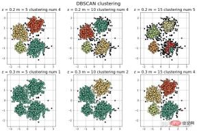
       -1, -1, -1, -1, -1, -1, -1, -1, -1, -1, -1, -1, -1])

2.DBSCAN

DBSCAN(노이즈가 있는 애플리케이션의 밀도 기반 공간 클러스터링) 원리

각 포인트를 중심으로 동네를 설정하고 동네에 필요한 포인트 수를 설정합니다. 샘플 포인트가 지정된 요구 사항보다 크면 해당 포인트가 동네의 포인트와 동일한 카테고리에 속하는 것으로 간주됩니다. .지정된 값보다 작을 경우 다른 점과 인접해 있는 A점이 경계점인 경우.

2.1 DBSCAN 데모

# 参考https://blog.csdn.net/hb707934728/article/details/71515160
#
# 官方示例 https://scikit-learn.org/stable/auto_examples/cluster/plot_dbscan.html#sphx-glr-auto-examples-cluster-plot-dbscan-py

import numpy as np

import matplotlib.pyplot as plt
import matplotlib.colors

import sklearn.datasets as ds
from sklearn.cluster import DBSCAN
from sklearn.preprocessing import StandardScaler


def expand(a, b):
    d = (b - a) * 0.1
    return a-d, b+d


if __name__ == "__main__":
    N = 1000
    centers = [[1, 2], [-1, -1], [1, -1], [-1, 1]]
    #scikit中的make_blobs方法常被用来生成聚类算法的测试数据，直观地说，make_blobs会根据用户指定的特征数量、
    # 中心点数量、范围等来生成几类数据，这些数据可用于测试聚类算法的效果。
    #函数原型：sklearn.datasets.make_blobs(n_samples=100, n_features=2,
    # centers=3, cluster_std=1.0, center_box=(-10.0, 10.0), shuffle=True, random_state=None)[source]
    #参数解析：
    # n_samples是待生成的样本的总数。
    #
    # n_features是每个样本的特征数。
    #
    # centers表示类别数。
    #
    # cluster_std表示每个类别的方差，例如我们希望生成2类数据，其中一类比另一类具有更大的方差，可以将cluster_std设置为[1.0, 3.0]。
    data, y = ds.make_blobs(N, n_features=2, centers=centers, cluster_std=[0.5, 0.25, 0.7, 0.5], random_state=0)
    data = StandardScaler().fit_transform(data)
    # 数据1的参数：(epsilon, min_sample)
    params = ((0.2, 5), (0.2, 10), (0.2, 15), (0.3, 5), (0.3, 10), (0.3, 15))

    plt.figure(figsize=(12, 8), facecolor='w')
    plt.suptitle(u'DBSCAN clustering', fontsize=20)

    for i in range(6):
        eps, min_samples = params[i]
        #参数含义：
        #eps:半径，表示以给定点P为中心的圆形邻域的范围
        #min_samples:以点P为中心的邻域内最少点的数量
        #如果满足,以点P为中心,半径为EPS的邻域内点的个数不少于MinPts,则称点P为核心点
        model = DBSCAN(eps=eps, min_samples=min_samples)
        model.fit(data)
        y_hat = model.labels_

        core_indices = np.zeros_like(y_hat, dtype=bool)  # 生成数据类型和数据shape和指定array一致的变量
        core_indices[model.core_sample_indices_] = True  # model.core_sample_indices_ border point位于y_hat中的下标

        # 统计总共有积累，其中为-1的为未分类样本
        y_unique = np.unique(y_hat)
        n_clusters = y_unique.size - (1 if -1 in y_hat else 0)
        print (y_unique, '聚类簇的个数为：', n_clusters)

        plt.subplot(2, 3, i+1) # 对第几个图绘制，2行3列，绘制第i+1个图
        # plt.cm.spectral https://blog.csdn.net/robin_Xu_shuai/article/details/79178857
        clrs = plt.cm.Spectral(np.linspace(0, 0.8, y_unique.size)) #用于给画图灰色
        for k, clr in zip(y_unique, clrs):
            cur = (y_hat == k)
            if k == -1:
                # 用于绘制未分类样本
                plt.scatter(data[cur, 0], data[cur, 1], s=20, c='k')
                continue
            # 绘制正常节点
            plt.scatter(data[cur, 0], data[cur, 1], s=30, c=clr, edgecolors='k')
            # 绘制边缘点
            plt.scatter(data[cur & core_indices][:, 0], data[cur & core_indices][:, 1], s=60, c=clr, marker='o', edgecolors='k')
        x1_min, x2_min = np.min(data, axis=0)
        x1_max, x2_max = np.max(data, axis=0)
        x1_min, x1_max = expand(x1_min, x1_max)
        x2_min, x2_max = expand(x2_min, x2_max)
        plt.xlim((x1_min, x1_max))
        plt.ylim((x2_min, x2_max))
        plt.grid(True)
        plt.title(u'$epsilon$ = %.1f m = %d clustering num %d'%(eps, min_samples, n_clusters), fontsize=16)
    plt.tight_layout()
    plt.subplots_adjust(top=0.9)
    plt.show()
[-1  0  1  2  3] 聚类簇的个数为： 4
[-1  0  1  2  3] 聚类簇的个数为： 4
[-1  0  1  2  3  4] 聚类簇的个数为： 5
[-1  0] 聚类簇的个数为： 1
[-1  0  1] 聚类簇的个数为： 2
[-1  0  1  2  3] 聚类簇的个数为： 4

2.2 사용자 정의 테스트 샘플 사용

#
# 参考https://blog.csdn.net/hb707934728/article/details/71515160
#
# 官方示例 https://scikit-learn.org/stable/auto_examples/cluster/plot_dbscan.html#sphx-glr-auto-examples-cluster-plot-dbscan-py

import numpy as np

import matplotlib.pyplot as plt
import matplotlib.colors

import sklearn.datasets as ds
from sklearn.cluster import DBSCAN
from sklearn.preprocessing import StandardScaler


def expand(a, b):
    d = (b - a) * 0.1
    return a-d, b+d


if __name__ == "__main__":
    N = 1000
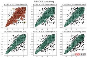
    data = X_train_demo.values
    # 数据1的参数：(epsilon, min_sample)
    params = ((0.2, 5), (0.2, 10), (0.2, 15), (0.2, 20), (0.2, 25), (0.2, 30))

    plt.figure(figsize=(12, 8), facecolor='w')
    plt.suptitle(u'DBSCAN clustering', fontsize=20)

    for i in range(6):
        eps, min_samples = params[i]
        #参数含义：
        #eps:半径，表示以给定点P为中心的圆形邻域的范围
        #min_samples:以点P为中心的邻域内最少点的数量
        #如果满足,以点P为中心,半径为EPS的邻域内点的个数不少于MinPts,则称点P为核心点
        model = DBSCAN(eps=eps, min_samples=min_samples)
        model.fit(data)
        y_hat = model.labels_

        core_indices = np.zeros_like(y_hat, dtype=bool)  # 生成数据类型和数据shape和指定array一致的变量
        core_indices[model.core_sample_indices_] = True  # model.core_sample_indices_ border point位于y_hat中的下标

        # 统计总共有积累，其中为-1的为未分类样本
        y_unique = np.unique(y_hat)
        n_clusters = y_unique.size - (1 if -1 in y_hat else 0)
        print (y_unique, '聚类簇的个数为：', n_clusters)

        plt.subplot(2, 3, i+1) # 对第几个图绘制，2行3列，绘制第i+1个图
        # plt.cm.spectral https://blog.csdn.net/robin_Xu_shuai/article/details/79178857
        clrs = plt.cm.Spectral(np.linspace(0, 0.8, y_unique.size)) #用于给画图灰色
        for k, clr in zip(y_unique, clrs):
            cur = (y_hat == k)
            if k == -1:
                # 用于绘制未分类样本
                plt.scatter(data[cur, 0], data[cur, 1], s=20, c='k')
                continue
            # 绘制正常节点
            plt.scatter(data[cur, 0], data[cur, 1], s=30, c=clr, edgecolors='k')
            # 绘制边缘点
            plt.scatter(data[cur & core_indices][:, 0], data[cur & core_indices][:, 1], s=60, c=clr, marker='o', edgecolors='k')
        x1_min, x2_min = np.min(data, axis=0)
        x1_max, x2_max = np.max(data, axis=0)
        x1_min, x1_max = expand(x1_min, x1_max)
        x2_min, x2_max = expand(x2_min, x2_max)
        plt.xlim((x1_min, x1_max))
        plt.ylim((x2_min, x2_max))
        plt.grid(True)
        plt.title(u'$epsilon$ = %.1f m = %d clustering num %d'%(eps, min_samples, n_clusters), fontsize=14)
    plt.tight_layout()
    plt.subplots_adjust(top=0.9)
    plt.show()

참고: 테스트 샘플의 양쪽 끝에서 DBSCAN이 "팁의 샘플 분류"에서 더 나은 성능을 발휘할 수 있음을 알 수 있습니다. .

2.3 핵심 코드

model = DBSCAN(eps=eps, min_samples=min_samples) # 분류기 구성

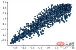
from sklearn.cluster import DBSCAN
from sklearn import metrics
data = X_train_demo.values
eps, min_samples = 0.2, 10
# eps为领域的大小，min_samples为领域内最小点的个数
model = DBSCAN(eps=eps, min_samples=min_samples) # 构造分类器
model.fit(data) # 拟合
labels = model.labels_ # 获取类别标签，-1表示未分类
# 获取其中的core points
core_indices = np.zeros_like(labels, dtype=bool)  # 生成数据类型和数据shape和指定array一致的变量
core_indices[model.core_sample_indices_] = True  # model.core_sample_indices_ border point位于labels中的下标
core_point = data[core_indices]
# 获取非异常点
normal_point = data[labels>=0]
# 绘制剔除了异常值后的图
plt.scatter(normal_point[:,0],normal_point[:,1],edgecolors='k')
plt.show()

2.4 필터 기능 구성

이 기능은 먼저 고정 매개변수를 사용하여 분석을 용이하게 하기 위해 표준화되었습니다

2.4.1 필터 기능

def filter_data(data0, params):
    from sklearn.cluster import DBSCAN
    from sklearn import metrics
    scaler = StandardScaler()
    scaler.fit(data0)
    data = scaler.transform(data0)

    eps, min_samples = params
    # eps为领域的大小，min_samples为领域内最小点的个数
    model = DBSCAN(eps=eps, min_samples=min_samples) # 构造分类器
    model.fit(data) # 拟合
    labels = model.labels_ # 获取类别标签，-1表示未分类
    # 获取其中的core points
    core_indices = np.zeros_like(labels, dtype=bool)  # 生成数据类型和数据shape和指定array一致的变量
    core_indices[model.core_sample_indices_] = True  # model.core_sample_indices_ border point位于labels中的下标
    core_point = data[core_indices]
    # 获取非异常点
    normal_point = data0[labels>=0]
    return normal_point

2.4.2 분류 결과 측정

(마크다운 형식 변환이 너무 귀찮아서 직접 스크린샷을 찍었습니다::>_<::>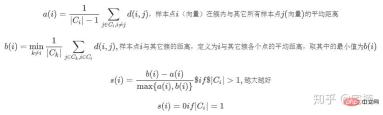

# 轮廓系数
metrics.silhouette_score(data, labels, metric='euclidean')
[out]0.13250260550638607
# Calinski-Harabaz Index 系数
metrics.calinski_harabaz_score(data, labels,)
[out]16.414158842632794

3.

# reference:https://scikit-learn.org/stable/auto_examples/svm/plot_oneclass.html#sphx-glr-auto-examples-svm-plot-oneclass-py

import numpy as np
import matplotlib.pyplot as plt
import matplotlib.font_manager
from sklearn import svm

xx, yy = np.meshgrid(np.linspace(-5, 5, 500), np.linspace(-5, 5, 500))
# Generate train data
X = 0.3 * np.random.randn(100, 2)
X_train = np.r_[X + 2, X - 2]
# Generate some regular novel observations
X = 0.3 * np.random.randn(20, 2)
X_test = np.r_[X + 2, X - 2]
# Generate some abnormal novel observations
X_outliers = np.random.uniform(low=-4, high=4, size=(20, 2))

# fit the model
clf = svm.OneClassSVM(nu=0.1, kernel="rbf", gamma=0.1)
clf.fit(X_train)
y_pred_train = clf.predict(X_train)
y_pred_test = clf.predict(X_test)
y_pred_outliers = clf.predict(X_outliers)
n_error_train = y_pred_train[y_pred_train == -1].size
n_error_test = y_pred_test[y_pred_test == -1].size
n_error_outliers = y_pred_outliers[y_pred_outliers == 1].size

# plot the line, the points, and the nearest vectors to the plane
Z = clf.decision_function(np.c_[xx.ravel(), yy.ravel()])
Z = Z.reshape(xx.shape)

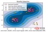
plt.title("Novelty Detection")
plt.contourf(xx, yy, Z, levels=np.linspace(Z.min(), 0, 7), cmap=plt.cm.PuBu)
a = plt.contour(xx, yy, Z, levels=[0], linewidths=2, colors='darkred')
plt.contourf(xx, yy, Z, levels=[0, Z.max()], colors='palevioletred')

s = 40
b1 = plt.scatter(X_train[:, 0], X_train[:, 1], c='white', s=s, edgecolors='k')
b2 = plt.scatter(X_test[:, 0], X_test[:, 1], c='blueviolet', s=s,
                 edgecolors='k')
c = plt.scatter(X_outliers[:, 0], X_outliers[:, 1], c='gold', s=s,
                edgecolors='k')
plt.axis('tight')
plt.xlim((-5, 5))
plt.ylim((-5, 5))
plt.legend([a.collections[0], b1, b2, c],
           ["learned frontier", "training observations",
            "new regular observations", "new abnormal observations"],
           loc="upper left",
           prop=matplotlib.font_manager.FontProperties(size=11))
plt.xlabel(
    "error train: %d/200 ; errors novel regular: %d/40 ; "
    "errors novel abnormal: %d/40"
    % (n_error_train, n_error_test, n_error_outliers))
plt.show()

3.2 핵심 코드

from sklearn import svm
X_train = X_train_demo.values
# 构造分类器
clf = svm.OneClassSVM(nu=0.2, kernel="rbf", gamma=0.2)
clf.fit(X_train)
# 预测，结果为-1或者1
labels = clf.predict(X_train)
# 分类分数
score = clf.decision_function(X_train) # 获取置信度
# 获取正常点
X_train_normal = X_train[labels>0]

아웃라이어 제거 전

아웃라이어 제거 후

plt.scatter(X_train_normal[:,0],X_train_normal[:,1])
plt.show()

4. LOF(Local Outlier Factor)

LOF는 샘플의 이상치를 계산하여 반영합니다. 수치적인 점수 . 이 값의 일반적인 의미는 다음과 같습니다.

샘플 포인트 주변 샘플 포인트의 평균 밀도가 샘플 포인트의 밀도보다 높습니다. 비율이 1보다 클수록 점 위치의 밀도는 주변 샘플 위치의 밀도보다 작습니다.

#
# 参考https://blog.csdn.net/hb707934728/article/details/71515160
#
# 官方示例 https://scikit-learn.org/stable/auto_examples/cluster/plot_dbscan.html#sphx-glr-auto-examples-cluster-plot-dbscan-py

import numpy as np

import matplotlib.pyplot as plt
import matplotlib.colors

from sklearn.neighbors import LocalOutlierFactor

def expand(a, b):
    d = (b - a) * 0.1
    return a-d, b+d


if __name__ == "__main__":
    N = 1000
    data = X_train_demo.values
    # 数据1的参数：(epsilon, min_sample)
    params = ((0.01, 5), (0.05, 10), (0.1, 15), (0.15, 20), (0.2, 25), (0.25, 30))

    plt.figure(figsize=(12, 8), facecolor='w')
    plt.suptitle(u'DBSCAN clustering', fontsize=20)

    for i in range(6):
        outliers_fraction, min_samples = params[i]
        #参数含义：
        #eps:半径，表示以给定点P为中心的圆形邻域的范围
        #min_samples:以点P为中心的邻域内最少点的数量
        #如果满足,以点P为中心,半径为EPS的邻域内点的个数不少于MinPts,则称点P为核心点

        model = LocalOutlierFactor(n_neighbors=min_samples, contamination=outliers_fraction)
        y_hat = model.fit_predict(X_train)

        # 统计总共有积累，其中为-1的为未分类样本
        y_unique = np.unique(y_hat)

        # clrs = []
        # for c in np.linspace(16711680, 255, y_unique.size):
        #     clrs.append('#%06x' % c)
        plt.subplot(2, 3, i+1) # 对第几个图绘制，2行3列，绘制第i+1个图
        # plt.cm.spectral https://blog.csdn.net/robin_Xu_shuai/article/details/79178857
        clrs = plt.cm.Spectral(np.linspace(0, 0.8, y_unique.size)) #用于给画图灰色
        for k, clr in zip(y_unique, clrs):
            cur = (y_hat == k)
            if k == -1:
                # 用于绘制未分类样本
                plt.scatter(data[cur, 0], data[cur, 1], s=20, c='k')
                continue
            # 绘制正常节点
            plt.scatter(data[cur, 0], data[cur, 1], s=30, c=clr, edgecolors='k')
        x1_max, x2_max = np.max(data, axis=0)
        x1_min, x2_min = np.min(data, axis=0)
        x1_min, x1_max = expand(x1_min, x1_max)
        x2_min, x2_max = expand(x2_min, x2_max)
        plt.xlim((x1_min, x1_max))
        plt.ylim((x2_min, x2_max))
        plt.grid(True)
        plt.title(u'outliers_fraction = %.1f min_samples = %d'%(outliers_fraction, min_samples), fontsize=12)
    plt.tight_layout()
    plt.subplots_adjust(top=0.9)
    plt.show()

4.1 핵심코드

from sklearn.neighbors import LocalOutlierFactor
X_train = X_train_demo.values
# 构造分类器
## 25个样本点为一组，异常值点比例为0.2
clf = LocalOutlierFactor(n_neighbors=25, contamination=0.2)
# 预测，结果为-1或者1
labels = clf.fit_predict(X_train)
# 获取正常点
X_train_normal = X_train[labels>0]

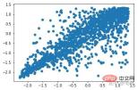
이상치 제거 전

plt.scatter(X_train[:,0],X_train[:,1])
plt.show()

이상치 제거 후

plt.scatter(X_train_normal[:,0],X_train_normal[:,1])
plt.show()

더 많은 컴퓨터 관련 지식은

FAQ

칼럼을 방문해 주세요!

위 내용은 비정상적인 데이터를 제거하는 네 가지 방법은 무엇입니까?의 상세 내용입니다. 자세한 내용은 PHP 중국어 웹사이트의 기타 관련 기사를 참조하세요!