


The article shows how to add colors to your data validation lists to make them more visually appealing and user-friendly.
You don't have to be an expert to make a drop-down menu in Excel or Google Sheets. But let's be honest - staring at a long list of values can be pretty boring. If you're looking to add some excitement to your spreadsheets, why not try highlighting a drop-down list with color? Whether you're organizing a list of products, categorizing expenses, or tracking sales data, a colored dropdown will make your data easier to read and understand. In this article, we'll show you how to do just that.

How to create Excel colored drop down list
If you use Excel for data entry, you've likely used the Data Validation feature to create drop-down lists. But did you know that you can also add colors to these lists? This section will guide you through the steps to colorize your drop-down list for a more eye-catching look.
Step 1. Create drop-down list
To add color to your Excel picklist, you first need to create the list itself. If you're unfamiliar with this process, refer to our separate article on creating a drop-down list that describes all possible methods in detail.
For this example, let's assume you have the source list of items in A3:A10 and you've created a drop-down menu with those items. To do that, simply select the range of cells where you want the dropdown to appear (D3:D12 in our case) and click the Data Validation button on the Data tab. In the Data Validation dialog box that appears, choose List from the Allow drop-down menu and, in the Source field, enter the reference to the range of cells containing your items.

Once you've created your drop-down list, you can move on to adding colors.
Step 2. Add colors to drop-down menu
To highlight your picklist with some color, we will be using Excel conditional formatting. The steps are:
- Select the cell(s) with your drop-down menu.
- On the Home tab, in the Styles group, click Conditional Formatting > New Rule… .
- In the New Formatting Rule dialog window, choose the Format only cells that contain option.
- Choose Specific Text from the first drop-down box and containing from the second drop-down box. In the third box, enter the reference to the cell containing the value that you want to format with a certain color like shown in the screenshot below. Alternatively, you can type the value enclosed in double quotes directly in the box, e.g. "Blue".

- Click the Format button.
- In the Format Cells dialog box, switch to the Fill tab, choose the color you like for that particular item, and click OK.
- Back in the New Formatting Rule dialog window, review the settings, and if everything looks good, click OK to save the changes.


Step 3. Test your colored drop-down list
To test your colored drop down menu, click on the arrow next to the cell. You should see the list of items you entered, with the first item highlighted in the chosen color:

Repeat the above steps for other selections and you will get a cohesive color scheme that makes it easy to visually distinguish between different selections.

Tips:
- If you've chosen dark fill colors for your drop-down list, selecting the white font color will make your options more readable. Similarly, if you've chosen light fill colors, using a dark font color will provide better contrast and readability.
- Don't be afraid to experiment with different color combinations to find the one that works best for your data!
- In Excel 365, you can use the brand new IMAGE function to create dropdown with pictures.
How to make Google Sheets drop down list with color
Google Sheets has become a go-to tool for many people. Like its Microsoft Excel counterpart, it offers the ability to create drop-down menus for easier data entry. With the latest version of Google spreadsheets, you no longer need to rely on conditional formatting tricks. Now, you can add colors to your data validation lists directly as you create them!
To create a colored drop-down list in Google Sheets, follow these steps:
- Select one or more cells where we want the dropdown list to appear.
- From the top toolbar, select Data and click Data validation.
- On the Data Validation rules pane, click Add rule.
- In the Criteria drop down menu, pick either the Dropdown or Dropdown from a range option.
- If you choose Dropdown, type your values in the Option 1 and Option 2 boxes, clicking the Add another item button as needed.
If you choose Dropdown from a range, type the range reference in the text field or use the Select Data Range button to pick the range. Either way, be sure to use absolute references with the $ sign to lock cell addresses such as e.g. =$D$4:$D$8.
- Once you've entered your options, it's time to add some color! Simply select the color you want for each item. If you need more tints than shown in the predefined palette, click Customize, and then choose a custom color.
- When you're finished, click the Done button.


There you have it - a colored drop-down menu that not only looks great, but also helps you organize and analyze your data more effectively.

How to create color-coded drop down list
In the first part of this tutorial, you learned how to create dropdown with colored text values. But what if you want to create a color-coded dropdown where only colors are visible, without any text values? This section will show you how to achieve that outcome. By selecting the same color for both the fill and font, you can create a monochromatic effect that is ideal for organizing data in a clear and concise way. Let's dive in and learn how to create a color coded dropdown list with hidden text values.
Color coded dropdown list in Excel
To make a color-coded dropdown in Excel worksheets, you set up conditional formatting rule as described in Adding colors to drop-down menu. When choosing the format, switch between the Fill and Font tabs and pick the same color on both.
Choosing the fill color:

Choosing the font color:

As a result, you will have a color-coded drop down list where each option is represented by a colored cell. This visual representation can be especially useful for data sets with a large number of categories or where color is a significant factor.

Color coded dropdown list in Google Sheets
To color code drop down list in Google Sheets, follow these steps. After adding background colors (Step 6), do the following:
- Click on the color you've added to a certain item, and then click Customize.
- On the Background tab, copy the Hex color code:
- On the Text tab, paste the copied hex code:


That's it! After following the steps outlined above, you'll have a color-coded dropdown menu effectively hiding the text values and leaving only the color swatches visible.

Note. Please remember that the purpose of visual communication is to enhance understanding, and different situations may require different visual cues to achieve that goal. Color codes are useful for representing data where the color is the primary indicator of meaning. However, if you need to provide additional context for each item, using different fill and font colors can be a more effective way to communicate this information visually.
In conclusion, adding color to drop-down lists in Excel and Google Sheets is a great way to enhance the visual appeal of your spreadsheets while also making them more functional and comprehensible. So go ahead and try it out, and see how color can transform your spreadsheets today!
Practice workbook for download
Excel color drop down list (.xlsx file) Google Sheets drop down list with color (online sheet)
위 내용은 Excel 및 Google 시트에서 컬러 드롭 다운 목록을 만드는 방법의 상세 내용입니다. 자세한 내용은 PHP 중국어 웹사이트의 기타 관련 기사를 참조하세요!

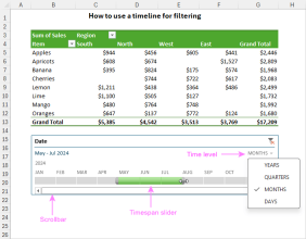 Excel에서 타임 라인을 작성하여 피벗 테이블 및 차트를 필터링하는 방법Mar 22, 2025 am 11:20 AM
이 기사에서는 Excel Pivot 테이블 및 차트 타임 라인을 작성하는 프로세스를 안내하고이를 사용하여 동적이고 매력적인 방식으로 데이터와 상호 작용하는 방법을 보여줍니다. 당신은 당신의 데이터를 pivo로 구성했습니다
 Excel에서 드롭 다운을하는 방법Mar 12, 2025 am 11:53 AM
이 기사에서는 단일 및 종속 목록을 포함하여 데이터 검증을 사용하여 Excel에서 드롭 다운 목록을 작성하는 방법을 설명합니다. 프로세스를 자세히 설명하고 일반적인 시나리오를위한 솔루션을 제공하며 데이터 입력 제한 및 PE와 같은 제한 사항에 대해 설명합니다.
 Excel에서 열을 합산하는 방법Mar 14, 2025 pm 02:42 PM
이 기사는 합 함수, 오토섬 기능 및 특정 세포를 합치하는 방법을 사용하여 Excel의 열을 합계하는 방법에 대해 설명합니다.
 엑셀에서 파이 차트를 만드는 방법Mar 14, 2025 pm 03:32 PM
이 기사에는 Excel에서 PIE 차트를 생성하고 사용자 정의하는 단계를 자세히 설명하여 시각적 분석을 향상시키기 위해 데이터 준비, 차트 삽입 및 개인화 옵션에 중점을 둡니다.
 Excel에서 테이블을 만드는 방법Mar 14, 2025 pm 02:53 PM
기사는 데이터 분석을 위해 합, 평균 및 피벗 테이블과 같은 함수를 사용하여 테이블을 작성, 서식 및 사용자 정의하고 설명합니다.
 Excel의 평균을 계산하는 방법Mar 14, 2025 pm 03:33 PM
기사는 평균 기능을 사용하여 Excel의 평균 계산에 대해 설명합니다. 주요 문제는 다른 데이터 세트 에이 기능을 효율적으로 사용하는 방법입니다. (158 자)
 Excel에 드롭 다운을 추가하는 방법Mar 14, 2025 pm 02:51 PM
기사는 데이터 검증을 사용하여 Excel에서 드롭 다운 목록 작성, 편집 및 제거에 대해 설명합니다. 주요 이슈 : 드롭 다운 목록을 효과적으로 관리하는 방법.
 Google 시트에 데이터를 정렬하기 위해 알아야 할 모든 것Mar 22, 2025 am 10:47 AM
Google 시트 분류 마스터 링 : 포괄적 인 가이드 Google 시트의 데이터 정렬은 복잡 할 필요가 없습니다. 이 안내서는 전체 시트를 정렬하는 것부터 특정 범위, 색상, 날짜 및 여러 열에 이르기까지 다양한 기술을 다룹니다. 당신이 노비이든


핫 AI 도구

Undresser.AI Undress
사실적인 누드 사진을 만들기 위한 AI 기반 앱

AI Clothes Remover
사진에서 옷을 제거하는 온라인 AI 도구입니다.

Undress AI Tool
무료로 이미지를 벗다

Clothoff.io
AI 옷 제거제

AI Hentai Generator
AI Hentai를 무료로 생성하십시오.

인기 기사
뜨거운 도구

SecList
SecLists는 최고의 보안 테스터의 동반자입니다. 보안 평가 시 자주 사용되는 다양한 유형의 목록을 한 곳에 모아 놓은 것입니다. SecLists는 보안 테스터에게 필요할 수 있는 모든 목록을 편리하게 제공하여 보안 테스트를 더욱 효율적이고 생산적으로 만드는 데 도움이 됩니다. 목록 유형에는 사용자 이름, 비밀번호, URL, 퍼징 페이로드, 민감한 데이터 패턴, 웹 셸 등이 포함됩니다. 테스터는 이 저장소를 새로운 테스트 시스템으로 간단히 가져올 수 있으며 필요한 모든 유형의 목록에 액세스할 수 있습니다.

에디트플러스 중국어 크랙 버전
작은 크기, 구문 강조, 코드 프롬프트 기능을 지원하지 않음

Eclipse용 SAP NetWeaver 서버 어댑터
Eclipse를 SAP NetWeaver 애플리케이션 서버와 통합합니다.

Atom Editor Mac 버전 다운로드
가장 인기 있는 오픈 소스 편집기

PhpStorm 맥 버전
최신(2018.2.1) 전문 PHP 통합 개발 도구

