Pythonでローパスフィルターぼかし画像関数を実装する方法

ローパス フィルターを使用して画像をぼかします

0.はじめに

ローパス フィルター(ローパス フィルター, LPF) は、画像の高周波部分をフィルターで除去し、低周波部分のみを通過させます。したがって、画像に LPF を適用すると、画像の詳細/エッジとノイズ/異常値が除去されます。このプロセスは、画像のぼかし (またはスムージング) とも呼ばれます。画像のスムージングは​​、複雑な画像処理タスクの前段階として使用できます。加工部分です。

1. 周波数領域におけるさまざまなタイプのカーネルとコンボリューション

1.1 画像ブラーの分類

画像ブラーには通常、次のタイプが含まれます:

• エッジブラー (エッジ) このタイプのブラーは通常、線形フィルター カーネルやガウス カーネルなどの畳み込みを通じて画像に明示的に適用されます。これらのフィルター カーネルを使用すると、画像内の不要なディテール/ノイズを平滑化/削除しました。

• モーション ブラー (Motion) は通常、画像をキャプチャするときの手ぶれ、つまりカメラまたは撮影対象が動いていることによって発生します。点広がり関数を使用して、このぼやけをシミュレートできます。

• 焦点ぼけブラー (de-focus) このタイプのブラーは、カメラで捉えたオブジェクトの焦点が合っていないときに発生します。ブラー ( Blur) カーネルを使用して、このブラーをシミュレートします。

次に、上記の 3 つの異なるタイプのカーネルを作成し、それらを画像に適用して、さまざまなタイプのカーネルが画像を処理した結果を観察します。

1.2 さまざまなカーネルを使用して画像ブラーを実行する

(1) まず、関数 get_gaussian_edge_blur_kernel() を定義して 2D## を返します。 # エッジブラーにはガウスブラーカーネルが使用されます。この関数は、ガウスの標準偏差 (σ; σ; σ) と、作成された 2D カーネルのサイズ (たとえば、sz = 15 でカーネルが作成されます) を受け入れます。関数のパラメータ。以下に示すように、最初に 1D ガウス カーネルが作成され、次に 2 つの 1D ガウス カーネルの外積が計算されて 2D カーネルが返されます。 #<pre class="brush:py;">import numpy as np import numpy.fft as fp from skimage.io import imread from skimage.color import rgb2gray import matplotlib.pyplot as plt import cv2 def get_gaussian_edge_blur_kernel(sigma, sz=15): # First create a 1-D Gaussian kernel x = np.linspace(-10, 10, sz) kernel_1d = np.exp(-x**2/sigma**2) kernel_1d /= np.trapz(kernel_1d) # normalize the sum to 1.0 # create a 2-D Gaussian kernel from the 1-D kernel kernel_2d = kernel_1d[:, np.newaxis] * kernel_1d[np.newaxis, :] return kernel_2d</pre>(2) 次に、関数

get_motion_blur_kernel()

を定義してモーション ブラー カーネルを生成し、指定された長さと特定の方向 (角度) のラインを取得します。画像の入力モーション ブラー エフェクトをシミュレートするためのコンボリューション カーネルとして使用します。

def get_motion_blur_kernel(ln, angle, sz=15):
    kern = np.ones((1, ln), np.float32)
    angle = -np.pi*angle/180
    c, s = np.cos(angle), np.sin(angle)
    A = np.float32([[c, -s, 0], [s, c, 0]])
    sz2 = sz // 2
    A[:,2] = (sz2, sz2) - np.dot(A[:,:2], ((ln-1)*0.5, 0))
    kern = cv2.warpAffine(kern, A, (sz, sz), flags=cv2.INTER_CUBIC)
    return kern

Functionget_motion_blur_kernel() は、ブラーの長さと角度、およびブラー カーネルのサイズをパラメータとして受け取ります。関数は

OpenCV

を使用します warpaffine() 関数は、カーネル行列を返します (行列の中心を中点とし、指定された長さと角度を使用してカーネルを取得します)。 (3) 最後に、関数 get_out_of_focus_kernel()

を定義して、焦点外カーネル (画像の焦点外ブラーをシミュレート) を生成します。コンボリューション カーネルとして指定された半径に基づいて円を作成します。この関数は、入力パラメーターとして半径

R (Deocus Radius) と生成されるカーネルのサイズを受け取ります。 <pre class="brush:py;"> def get_out_of_focus_kernel(r, sz=15): kern = np.zeros((sz, sz), np.uint8) cv2.circle(kern, (sz, sz), r, 255, -1, cv2.LINE_AA, shift=1) kern = np.float32(kern) / 255 return kern</pre>(4) 次に、関数 dft_convolve() を実装します。これは、画像の要素ごとの乗算と周波数領域のコンボリューション カーネルを使用して周波数領域コンボリューションを実行します (畳み込み定理に基づく）。この関数は、入力イメージ、カーネル、畳み込み計算の結果として得られる出力イメージもプロットします。

def dft_convolve(im, kernel):
    F_im = fp.fft2(im)
    #F_kernel = fp.fft2(kernel, s=im.shape)
    F_kernel = fp.fft2(fp.ifftshift(kernel), s=im.shape)
    F_filtered = F_im * F_kernel
    im_filtered = fp.ifft2(F_filtered)
    cmap = 'RdBu'
    plt.figure(figsize=(20,10))
    plt.gray()
    plt.subplot(131), plt.imshow(im), plt.axis('off'), plt.title('input image', size=10)
    plt.subplot(132), plt.imshow(kernel, cmap=cmap), plt.title('kernel', size=10)
    plt.subplot(133), plt.imshow(im_filtered.real), plt.axis('off'), plt.title('output image', size=10)
    plt.tight_layout()
    plt.show()

(5) get_gaussian_edge_blur_kernel() カーネル関数を適用します。を画像に適用し、入力、カーネル、出力ブラー イメージをプロットします。

im = rgb2gray(imread('3.jpg'))

kernel = get_gaussian_edge_blur_kernel(25, 25)
dft_convolve(im, kernel)

(6) 次に、get_motion_blur_kernel() 関数を画像に適用してプロットします。入力、カーネル、出力のぼやけた画像:

kernel = get_motion_blur_kernel(30, 60, 25)
dft_convolve(im, kernel)

(7) 最後に、get_out_of_focus_kernel() 関数を画像に適用し、入力、カーネル、出力を描画します。ぼやけた画像:

kernel = get_out_of_focus_kernel(15, 20)
dft_convolve(im, kernel)

2. scipy.ndimage フィルターを使用して画像をぼかしますscipy.ndimage このモジュールは、ローパスを適用できる一連の関数を提供します。周波数領域で画像にフィルターを適用します。このセクションでは、いくつかの例を通してこれらのフィルターの使用方法を学びます。

2.1 fourier_gaussian() 関数の使用

scipy.ndimage ライブラリの

fourier_gaussian()

関数を使用して、ガウス分布を使用してボリュームを実行します。周波数領域の累積演算におけるカーネル。

(1) まず、入力画像を読み取り、グレースケール画像に変換し、FFT:

import numpy as np
import numpy.fft as fp
from skimage.io import imread
import matplotlib.pyplot as plt
from scipy import ndimage

im = imread('1.png', as_gray=True)
freq = fp.fft2(im)

# を使用してその周波数領域表現を取得します。

##(2) 次に、fourier_gaussian() 関数を使用して、標準偏差が異なる 2 つのガウス カーネルを使用して画像に対してぼかし操作を実行し、入力画像、出力画像、およびパワースペクトル:

fig, axes = plt.subplots(2, 3, figsize=(20,15))
plt.subplots_adjust(0,0,1,0.95,0.05,0.05)
plt.gray() # show the filtered result in grayscale
axes[0, 0].imshow(im), axes[0, 0].set_title('Original Image', size=10)
axes[1, 0].imshow((20*np.log10( 0.1 + fp.fftshift(freq))).real.astype(int)), axes[1, 0].set_title('Original Image Spectrum', size=10)
i = 1
for sigma in [3,5]:
    convolved_freq = ndimage.fourier_gaussian(freq, sigma=sigma)
    convolved = fp.ifft2(convolved_freq).real # the imaginary part is an artifact
    axes[0, i].imshow(convolved)
    axes[0, i].set_title(r'Output with FFT Gaussian Blur, $\sigma$={}'.format(sigma), size=10)
    axes[1, i].imshow((20*np.log10( 0.1 + fp.fftshift(convolved_freq))).real.astype(int))
    axes[1, i].set_title(r'Spectrum with FFT Gaussian Blur, $\sigma$={}'.format(sigma), size=10)
    i += 1
for a in axes.ravel():
    a.axis('off')    
plt.show()

2.2 fourier_uniform() 関数を使用します

scipy.ndimage モジュール fourier_uniform()

の関数は、マルチ次元均一フーリエフィルター。周波数配列は、指定されたサイズの正方形カーネルのフーリエ変換によって乗算されます。次に、

LPF

(平均フィルター) を使用して入力グレースケール画像をぼかす方法を学びます。

(1) まず、入力画像を読み取り、DFT を使用してその周波数領域表現を取得します。<pre class="brush:py;">im = imread(&amp;#39;1.png&amp;#39;, as_gray=True) freq = fp.fft2(im)</pre><p><strong>(2)</strong> 然后，使用函数 <code>fourier_uniform() 应用 10x10 方形核(由功率谱上的参数指定)，以获取平滑输出：

freq_uniform = ndimage.fourier_uniform(freq, size=10)

(3) 绘制原始输入图像和模糊后的图像：

fig, (axes1, axes2) = plt.subplots(1, 2, figsize=(20,10))
plt.gray() # show the result in grayscale
im1 = fp.ifft2(freq_uniform)
axes1.imshow(im), axes1.axis('off')
axes1.set_title('Original Image', size=10)
axes2.imshow(im1.real) # the imaginary part is an artifact
axes2.axis('off')
axes2.set_title('Blurred Image with Fourier Uniform', size=10)
plt.tight_layout()
plt.show()

(4) 最后，绘制显示方形核的功率谱：

plt.figure(figsize=(10,10))
plt.imshow( (20*np.log10( 0.1 + fp.fftshift(freq_uniform))).real.astype(int))
plt.title('Frequency Spectrum with fourier uniform', size=10)
plt.show()

2.3 使用 fourier_ellipsoid() 函数

与上一小节类似，通过将方形核修改为椭圆形核，我们可以使用椭圆形核生成模糊的输出图像。

(1) 类似的，我们首先在图像的功率谱上应用函数 fourier_ellipsoid()，并使用 IDFT 在空间域中获得模糊后的输出图像：

freq_ellipsoid = ndimage.fourier_ellipsoid(freq, size=10)
im1 = fp.ifft2(freq_ellipsoid)

(2) 接下来，绘制原始输入图像和模糊后的图像：

fig, (axes1, axes2) = plt.subplots(1, 2, figsize=(20,10))
axes1.imshow(im), axes1.axis('off')
axes1.set_title('Original Image', size=10)
axes2.imshow(im1.real) # the imaginary part is an artifact
axes2.axis('off')
axes2.set_title('Blurred Image with Fourier Ellipsoid', size=10)
plt.tight_layout()
plt.show()

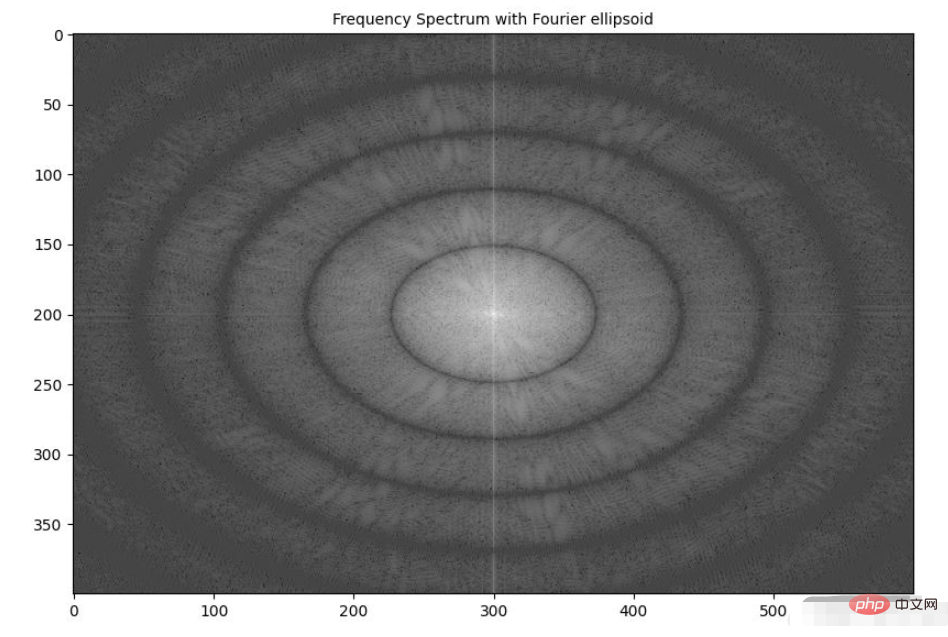
(3) 最后，显示应用椭圆形核后图像的频谱：

plt.figure(figsize=(10,10))
plt.imshow( (20*np.log10( 0.1 + fp.fftshift(freq_ellipsoid))).real.astype(int))
plt.title('Frequency Spectrum with Fourier ellipsoid', size=10)
plt.show()

3. 使用 scipy.fftpack 实现高斯模糊

我们已经学习了如何在实际应用中使用 numpy.fft 模块的 2D-FFT。在本节中，我们将介绍 scipy.fftpack 模块的 fft2() 函数用于实现高斯模糊。

(1) 使用灰度图像作为输入，并使用 FFT 从图像中创建 2D 频率响应数组：

import numpy as np
import numpy.fft as fp
from skimage.color import rgb2gray
from skimage.io import imread
import matplotlib.pyplot as plt
from scipy import signal
from matplotlib.ticker import LinearLocator, FormatStrFormatter

im = rgb2gray(imread('1.png'))
freq = fp.fft2(im)

(2) 通过计算两个 1D 高斯核的外积，在空间域中创建高斯 2D 核用作 LPF：

kernel = np.outer(signal.gaussian(im.shape[0], 1), signal.gaussian(im.shape[1], 1))

(3) 使用 DFT 获得高斯核的频率响应：

freq_kernel = fp.fft2(fp.ifftshift(kernel))

(4) 使用卷积定理通过逐元素乘法在频域中将 LPF 与输入图像卷积：

convolved = freq*freq_kernel # by the Convolution theorem

(5) 使用 IFFT 获得输出图像，需要注意的是，要正确显示输出图像，需要缩放输出图像：

im_blur = fp.ifft2(convolved).real
im_blur = 255 * im_blur / np.max(im_blur)

(6) 绘制图像、高斯核和在频域中卷积后获得图像的功率谱，可以使用 matplotlib.colormap 绘制色，以了解不同坐标下的频率响应值：

plt.figure(figsize=(20,20))
plt.subplot(221), plt.imshow(kernel, cmap='coolwarm'), plt.colorbar()
plt.title('Gaussian Blur Kernel', size=10)
plt.subplot(222)
plt.imshow( (20*np.log10( 0.01 + fp.fftshift(freq_kernel))).real.astype(int), cmap='inferno')
plt.colorbar()
plt.title('Gaussian Blur Kernel (Freq. Spec.)', size=10)
plt.subplot(223), plt.imshow(im, cmap='gray'), plt.axis('off'), plt.title('Input Image', size=10)
plt.subplot(224), plt.imshow(im_blur, cmap='gray'), plt.axis('off'), plt.title('Output Blurred Image', size=10)
plt.tight_layout()
plt.show()

(7) 要绘制输入/输出图像和 3D 核的功率谱，我们定义函数 plot_3d()，使用 mpl_toolkits.mplot3d 模块的 plot_surface() 函数获取 3D 功率谱图，给定相应的 Y 和Z值作为 2D 阵列传递：

def plot_3d(X, Y, Z, cmap=plt.cm.seismic):
    fig = plt.figure(figsize=(20,20))
    ax = fig.gca(projection='3d')
    # Plot the surface.
    surf = ax.plot_surface(X, Y, Z, cmap=cmap, linewidth=5, antialiased=False)
    #ax.plot_wireframe(X, Y, Z, rstride=10, cstride=10)
    #ax.set_zscale("log", nonposx='clip')
    #ax.zaxis.set_scale('log')
    ax.zaxis.set_major_locator(LinearLocator(10))
    ax.zaxis.set_major_formatter(FormatStrFormatter('%.02f'))
    ax.set_xlabel('F1', size=15)
    ax.set_ylabel('F2', size=15)
    ax.set_zlabel('Freq Response', size=15)
    #ax.set_zlim((-40,10))
    # Add a color bar which maps values to colors.
    fig.colorbar(surf) #, shrink=0.15, aspect=10)
    #plt.title('Frequency Response of the Gaussian Kernel')
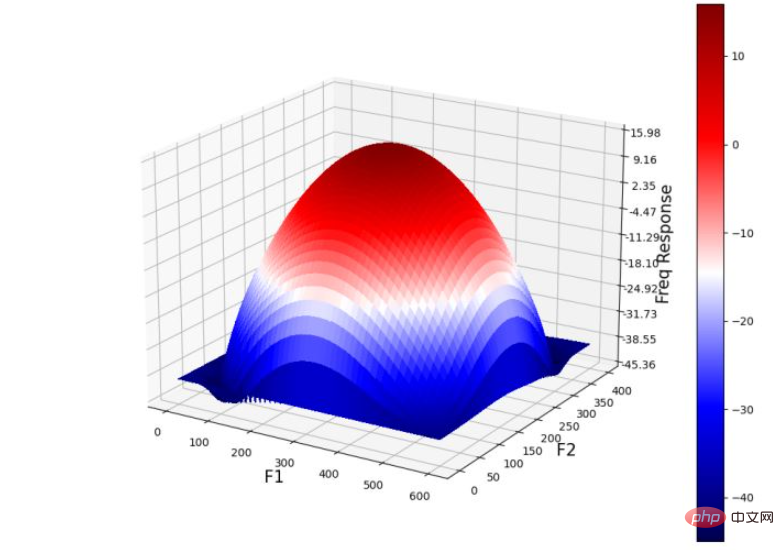
    plt.show()

(8) 在 3D 空间中绘制高斯核的频率响应，并使用 plot_3d() 函数：

Y = np.arange(freq.shape[0]) #-freq.shape[0]//2,freq.shape[0]-freq.shape[0]//2)
X = np.arange(freq.shape[1]) #-freq.shape[1]//2,freq.shape[1]-freq.shape[1]//2)
X, Y = np.meshgrid(X, Y)
Z = (20*np.log10( 0.01 + fp.fftshift(freq_kernel))).real
plot_3d(X,Y,Z)

下图显示了 3D 空间中高斯 LPF 核的功率谱：

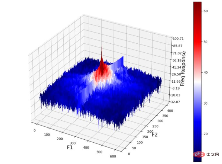
(9) 绘制 3D 空间中输入图像的功率谱：

Z = (20*np.log10( 0.01 + fp.fftshift(freq))).real
plot_3d(X,Y,Z)

(10) 最后，绘制输出图像的功率谱(通过将高斯核与输入图像卷积获得)：

Z = (20*np.log10( 0.01 + fp.fftshift(convolved))).real
plot_3d(X,Y,Z)

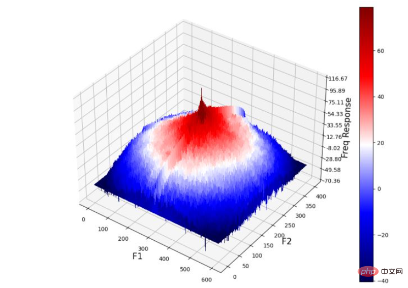
从输出图像的频率响应中可以看出，高频组件被衰减，从而导致细节的平滑/丢失，并导致输出图像模糊。

4. 彩色图像频域卷积

在本节中，我们将学习使用 scipy.signal 模块的 fftconvolve() 函数，用于与 RGB 彩色输入图像进行频域卷积，从而生成 RGB 彩色模糊输出图像：

scipy.signal.fftconvolve(in1, in2, mode='full', axes=None)

函数使用 FFT 卷积两个 n 维数组 in1 和 in2，并由 mode 参数确定输出大小。卷积模式 mode 具有以下类型：

• 输出是输入的完全离散线性卷积，默认情况下使用此种卷积模式

• 输出仅由那些不依赖零填充的元素组成，in1 或 in2 的尺寸必须相同

• 输出的大小与 in1 相同，并以输出为中心

4.1 基于 scipy.signal 模块的彩色图像频域卷积

接下来，我们实现高斯低通滤波器并使用 Laplacian 高通滤波器执行相应操作。

(1) 首先，导入所需的包，并读取输入 RGB 图像：

from skimage import img_as_float
from scipy import signal
import numpy as np
import matplotlib.pyplot as plt

im = img_as_float(plt.imread('1.png'))

(2) 实现函数 get_gaussian_edge_kernel()，并根据此函数创建一个尺寸为 15x15 的高斯核：

def get_gaussian_edge_blur_kernel(sigma, sz=15):
    # First create a 1-D Gaussian kernel
    x = np.linspace(-10, 10, sz)
    kernel_1d = np.exp(-x**2/sigma**2)
    kernel_1d /= np.trapz(kernel_1d) # normalize the sum to 1.0
    # create a 2-D Gaussian kernel from the 1-D kernel
    kernel_2d = kernel_1d[:, np.newaxis] * kernel_1d[np.newaxis, :]
    return kernel_2d
kernel = get_gaussian_edge_blur_kernel(sigma=10, sz=15)

(3) 然后，使用 np.newaxis 将核尺寸重塑为 15x15x1，并使用 same 模式调用函数 signal.fftconvolve()：

im1 = signal.fftconvolve(im, kernel[:, :, np.newaxis], mode='same')
im1 = im1 / np.max(im1)

在以上代码中使用的 mode='same'，可以强制输出形状与输入阵列形状相同，以避免边框效应。

(4) 接下来，使用 laplacian HPF 内核，并使用相同函数执行频域卷积。需要注意的是，我们可能需要缩放/裁剪输出图像以使输出值保持像素的浮点值范围 [0,1] 内：

kernel = np.array([[0,-1,0],[-1,4,-1],[0,-1,0]])
im2 = signal.fftconvolve(im, kernel[:, :, np.newaxis], mode='same')
im2 = im2 / np.max(im2)
im2 = np.clip(im2, 0, 1)

(5) 最后，绘制输入图像和使用卷积创建的输出图像。

plt.figure(figsize=(20,10))
plt.subplot(131), plt.imshow(im), plt.axis('off'), plt.title('original image', size=10)
plt.subplot(132), plt.imshow(im1), plt.axis('off'), plt.title('output with Gaussian LPF', size=10)
plt.subplot(133), plt.imshow(im2), plt.axis('off'), plt.title('output with Laplacian HPF', size=10)
plt.tight_layout()
plt.show()

以上がPythonでローパスフィルターぼかし画像関数を実装する方法の詳細内容です。詳細については、PHP 中国語 Web サイトの他の関連記事を参照してください。