物理学における二重バネ質量エネルギー系を解くための Python コード例

この記事では主に、Python を使用して物理学における二重バネ質量エネルギー系を解く方法に関する関連情報をサンプル コードを通じて詳しく紹介します。この記事は、あらゆる人の学習や仕事に役立つ特定の学習価値があります。友達が必要なので、編集者をフォローして一緒に学びましょう。

前書き

この記事では主に、物理学における二重バネ質量エネルギー系を解くための Python の使用に関する関連コンテンツを紹介し、参考と学習のために共有します。以下では多くは述べません。 、詳しく紹介していきましょう。

物理モデルは次のとおりです:

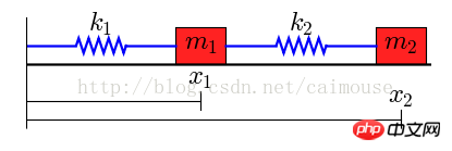
このシステムには 2 つのオブジェクトがあり、それらの質量はそれぞれ m1 と m2 で、2 つのバネで接続されています。伸縮システムは k1 と k2 (左端) です。修理済み。外力がないと仮定すると、2つのバネの長さはL1、L2となります。

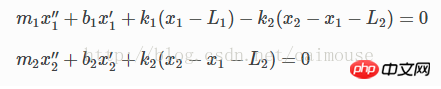
2つの物体には重力があるため、平面上では摩擦が生じ、摩擦係数はそれぞれb1、b2となります。したがって、次のように微分方程式を書くことができます:

これは 2 階の微分方程式です。Python を使用して解くには、1 階の微分方程式に変換する必要があります。したがって、次の 2 つの変数が導入されます:

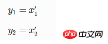
これら 2 つは移動速度に相当します。

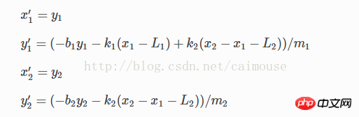
という操作でこれに変更できます。このとき、一次方程式はベクトル配列に変更でき、Pythonを使用して定義できます。コードは次のとおりです。

# Use ODEINT to solve the differential equations defined by the vector field 
from scipy.integrate import odeint 
 
def vectorfield(w, t, p): 
 """ 
 Defines the differential equations for the coupled spring-mass system. 
 
 Arguments: 
  w : vector of the state variables: 
     w = [x1,y1,x2,y2] 
  t : time 
  p : vector of the parameters: 
     p = [m1,m2,k1,k2,L1,L2,b1,b2] 
 """ 
 x1, y1, x2, y2 = w 
 m1, m2, k1, k2, L1, L2, b1, b2 = p 
 
 # Create f = (x1',y1',x2',y2'): 
 f = [y1, 
   (-b1 * y1 - k1 * (x1 - L1) + k2 * (x2 - x1 - L2)) / m1, 
   y2, 
   (-b2 * y2 - k2 * (x2 - x1 - L2)) / m2] 
 return f 
 
# Parameter values 
# Masses: 
m1 = 1.0 
m2 = 1.5 
# Spring constants 
k1 = 8.0 
k2 = 40.0 
# Natural lengths 
L1 = 0.5 
L2 = 1.0 
# Friction coefficients 
b1 = 0.8 
b2 = 0.5 
 
# Initial conditions 
# x1 and x2 are the initial displacements; y1 and y2 are the initial velocities 
x1 = 0.5 
y1 = 0.0 
x2 = 2.25 
y2 = 0.0 
 
# ODE solver parameters 
abserr = 1.0e-8 
relerr = 1.0e-6 
stoptime = 10.0 
numpoints = 250 
 
# Create the time samples for the output of the ODE solver. 
# I use a large number of points, only because I want to make 
# a plot of the solution that looks nice. 
t = [stoptime * float(i) / (numpoints - 1) for i in range(numpoints)] 
 
# Pack up the parameters and initial conditions: 
p = [m1, m2, k1, k2, L1, L2, b1, b2] 
w0 = [x1, y1, x2, y2] 
 
# Call the ODE solver. 
wsol = odeint(vectorfield, w0, t, args=(p,), 
    atol=abserr, rtol=relerr) 
 
with open('two_springs.dat', 'w') as f: 
 # Print & save the solution. 
 for t1, w1 in zip(t, wsol):   
  out = '{0} {1} {2} {3} {4}\n'.format(t1, w1[0], w1[1], w1[2], w1[3]); 
  print(out) 
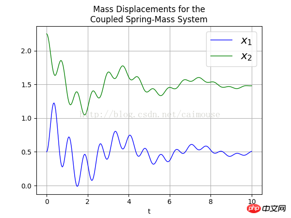
  f.write(out);

ここに結果を出力します ファイル two_springs.dat に移動し、データを画像として表示するプログラムを作成すると、論文を公開できます。 コードは次のとおりです。

# Plot the solution that was generated 
 
from numpy import loadtxt 
from pylab import figure, plot, xlabel, grid, hold, legend, title, savefig 
from matplotlib.font_manager import FontProperties 
 
t, x1, xy, x2, y2 = loadtxt('two_springs.dat', unpack=True) 
 
figure(1, figsize=(6, 4.5)) 
 
xlabel('t') 
grid(True) 
lw = 1 
 
plot(t, x1, 'b', linewidth=lw) 
plot(t, x2, 'g', linewidth=lw) 
 
legend((r'$x_1$', r'$x_2$'), prop=FontProperties(size=16)) 
title('Mass Displacements for the\nCoupled Spring-Mass System') 
savefig('two_springs.png', dpi=100)

最後に、次のように出力された PNG 画像を確認してみましょう:

概要

以上が物理学における二重バネ質量エネルギー系を解くための Python コード例の詳細内容です。詳細については、PHP 中国語 Web サイトの他の関連記事を参照してください。