


2 つの頂点間の最短パスは、合計重みが最小のパスです。
エッジに非負の重みを持つグラフを与えて、2 つの頂点間の最短経路を見つけるためのよく知られたアルゴリズムは、オランダのコンピューター科学者である Edsger Dijkstra によって発見されました。頂点 s から頂点 v までの最短経路を見つけるために、ダイクストラのアルゴリズム は s からすべての頂点までの最短経路を見つけます。したがって、ダイクストラのアルゴリズムは、単一ソースの最短経路アルゴリズムとして知られています。このアルゴリズムは、cost[v]を使用して、頂点vからソース頂点sまでの最短パスのコストを保存します。 コスト[s]は0です。最初に、他のすべての頂点の cost[v] に無限大を割り当てます。このアルゴリズムは、V – T で最小の コスト[u] を持つ頂点 u を繰り返し見つけ、u を T に移動します。 .
アルゴリズムは以下のコードで説明されています。
Input: a graph G = (V, E) with non-negative weights
Output: a shortest path tree with the source vertex s as the root
 1 ShortestPathTree getShortestPath(s) {
 2 Let T be a set that contains the vertices whose
 3 paths to s are known; Initially T is empty;
 4 Set cost[s] = 0; and cost[v] = infinity for all other vertices in V;
 5
 6 while (size of T  cost[u] + w(u, v)) {
11 cost[v] = cost[u] + w(u, v); parent[v] = u;
12 }
13 }
14 }
このアルゴリズムは、最小スパニング ツリーを見つけるための Prim のアルゴリズムに非常に似ています。どちらのアルゴリズムも、頂点を T と V - T の 2 つのセットに分割します。 Prim のアルゴリズムの場合、set T には、すでにツリーに追加されている頂点が含まれます。ダイクストラの場合、セット T には、ソースへの最短パスが見つかった頂点が含まれます。どちらのアルゴリズムも、V – T から頂点を繰り返し見つけて、それを T に追加します。プリムのアルゴリズムの場合、頂点は、エッジの重みが最小であるセット内のいくつかの頂点に隣接します。ダイクストラのアルゴリズムでは、頂点はソースへの総コストが最小となるセット内のいくつかの頂点に隣接します。
アルゴリズムは、cost[s] を 0 に設定することから始まり (4 行目)、他のすべての頂点の cost[v] を無限大に設定します。次に、最小の コスト[u]で V – T から T に頂点 (u とします) を継続的に追加します (7 行目 – 8)、以下の図に示すように。 u を T に追加した後、アルゴリズムは各 vcost[v] と parent[v] を更新します。 > (u, v) が T かつ cost[v] > にある場合、T にはありません。 cost[u] + w(u, v) (10 ~ 11 行目).

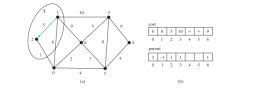
1 であるとします。したがって、cost[1] = 0 であり、下の図 b に示すように、他のすべての頂点のコストは最初は ∞ です。 parent[i] を使用して、パス内の i の親を示します。便宜上、ソース ノードの親を -1 に設定します。

Tは空です。アルゴリズムはコストが最小の頂点を選択します。この場合、頂点は 1 です。以下の図に示すように、アルゴリズムは 1 を T に加算します。その後、1 に隣接する各頂点のコストを調整します。以下の図 b に示すように、頂点 2、0、6、3 とその親のコストが更新されます。

2、0、6、および 3 はソース頂点に隣接しており、頂点 2 は V-T 内のコストが最小のものであるため、以下の図に示すように 2 を T に追加し、頂点のコストと親を更新します。 V-T であり、2 に隣接しています。 cost[0] は 6 に更新され、その親は 2 に設定されます。 1 から 2 への矢印線は、2 が 2 に追加された後、1 が 2 の親であることを示します。 た
.
現在、T には {1、2} が含まれています。頂点 0 はコストが最小の V-T の頂点であるため、以下の図に示すように 0 を T に追加し、 V-T 内で、該当する場合は 0 に隣接する頂点のコストと親。 cost[5] は 10 に更新され、その親は 0 に設定され、cost[6] は 8 であり、その親は 0 に設定されています。

T には {1、2、0} が含まれています。頂点 6 はコストが最小の V-T の頂点であるため、以下の図に示すように 6 を T に追加し、該当する場合、V-T および 6 に隣接する頂点のコストと親。

T には {1、2、0、6} が含まれています。頂点 3 または 5 は、V-T 内でコストが最も小さい頂点です。 3 または 5 を T に追加できます。以下の図に示すように、3 を T に追加し、V-T 内で 3 に隣接する頂点のコストと親を更新しましょう。該当する場合。 cost[4] は 18 に更新され、その親は 3 に設定されます。

T には、{1、2、0、6、3}。頂点 5 はコストが最小の V-T の頂点であるため、以下の図に示すように 5 を T に追加し、 V-T 内にあり、該当する場合は 5 に隣接する頂点のコストと親。 cost[4] は 10 に更新され、その親は 5 に設定されます。
 現在、
現在、
には、{1、2、0、6、3、5}。 V-T 内の頂点 4 はコストが最小の頂点であるため、下の図に示すように 4 を T に追加します。
ご覧のとおり、アルゴリズムは基本的にソース頂点からのすべての最短パスを検索し、ソース頂点をルートとするツリーを生成します。このツリーを  単一ソースの全最短パス ツリー
最短パス ツリー) と呼びます。このツリーをモデル化するには、以下の図に示すように、Tree クラスを拡張する ShortestPathTree という名前のクラスを定義します。 ShortestPathTree は、WeightedGraph.java. の行 200 ~ 224 で WeightedGraph の内部クラスとして定義されています。
 getShortestPath(int sourceVertex)
cost[sourceVertex] を 0 に設定し (162 行目)、他のすべての頂点の cost[v] を無限大に設定します (159 ~ 161 行目)。 sourceVertex の親は -1 に設定されます (166 行目)。 T は、最短パス ツリーに追加された頂点を格納するリストです (169 行目)。 T に追加された頂点の順序を記録するために、セットではなく T のリストを使用します。 最初、T
は空です。T を展開するには、メソッドは次の操作を実行します。
- Find the vertex u with the smallest cost[u] (lines 175–181) and add it into T (line 183).
- After adding u in T, update cost[v] and parent[v] for each v adjacent to u in V-T if cost[v] > cost[u] + w(u, v) (lines 186–192).
Once all vertices from s are added to T, an instance of ShortestPathTree is created (line 196).
The ShortestPathTree class extends the Tree class (line 200). To create an instance of ShortestPathTree, pass sourceVertex, parent, T, and cost (lines 204–205). sourceVertex becomes the root in the tree. The data fields root, parent, and searchOrder are defined in the Tree class, which is an inner class defined in AbstractGraph.
Note that testing whether a vertex i is in T by invoking T.contains(i) takes O(n) time, since T is a list. Therefore, the overall time complexity for this implemention is O(n^3).
Dijkstra’s algorithm is a combination of a greedy algorithm and dynamic programming. It is a greedy algorithm in the sense that it always adds a new vertex that has the shortest distance to the source. It stores the shortest distance of each known vertex to the source and uses it later to avoid redundant computing, so Dijkstra’s algorithm also uses dynamic programming.
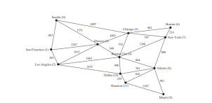
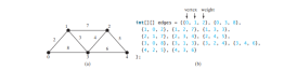
The code below gives a test program that displays the shortest paths from Chicago to all other cities in Figure below and the shortest paths from vertex 3 to all vertices for the graph in Figure below a, respectively.
package demo;

public class TestShortestPath {

    public static void main(String[] args) {
String[] vertices = {"Seattle", "San Francisco", "Los Angeles", "Denver", "Kansas City", "Chicago", "Boston", "New York", "Atlanta", "Miami", "Dallas", "Houston"};

        int[][] edges = {
                {0, 1, 807}, {0, 3, 1331}, {0, 5, 2097},
                {1, 0, 807}, {1, 2, 381}, {1, 3, 1267},
                {2, 1, 381}, {2, 3, 1015}, {2, 4, 1663}, {2, 10, 1435},
                {3, 0, 1331}, {3, 1, 1267}, {3, 2, 1015}, {3, 4, 599}, {3, 5, 1003},
                {4, 2, 1663}, {4, 3, 599}, {4, 5, 533}, {4, 7, 1260}, {4, 8, 864}, {4, 10, 496},
                {5, 0, 2097}, {5, 3, 1003}, {5, 4, 533}, {5, 6, 983}, {5, 7, 787},
                {6, 5, 983}, {6, 7, 214},
                {7, 4, 1260}, {7, 5, 787}, {7, 6, 214}, {7, 8, 888},
                {8, 4, 864}, {8, 7, 888}, {8, 9, 661}, {8, 10, 781}, {8, 11, 810},
                {9, 8, 661}, {9, 11, 1187},
                {10, 2, 1435}, {10, 4, 496}, {10, 8, 781}, {10, 11, 239},
                {11, 8, 810}, {11, 9, 1187}, {11, 10, 239}
        };

        WeightedGraph<string> graph1 = new WeightedGraph(vertices, edges);
        WeightedGraph<string>.ShortestPathTree tree1 = graph1.getShortestPath(graph1.getIndex("Chicago"));
        tree1.printAllPaths();

        // Display shortest paths from Houston to Chicago
        System.out.println("Shortest path from Houston to Chicago: ");
        java.util.List<string> path = tree1.getPath(graph1.getIndex("Houston"));
        for(String s: path) {
            System.out.print(s + " ");
        }

        edges = new int[][]{
            {0, 1, 2}, {0, 3, 8},
            {1, 0, 2}, {1, 2, 7}, {1, 3, 3},
            {2, 1, 7}, {2, 3, 4}, {2, 4, 5},
            {3, 0, 8}, {3, 1, 3}, {3, 2, 4}, {3, 4, 6},
            {4, 2, 5}, {4, 3, 6}
        };

        WeightedGraph<integer> graph2 = new WeightedGraph(edges, 5);
        WeightedGraph<integer>.ShortestPathTree tree2 = graph2.getShortestPath(3);
        System.out.println("\n");
        tree2.printAllPaths();
    }

}

</integer></integer></string></string></string>
All shortest paths from Chicago are:
A path from Chicago to Seattle: Chicago Seattle (cost: 2097.0)
A path from Chicago to San Francisco:
Chicago Denver San Francisco (cost: 2270.0)
A path from Chicago to Los Angeles:
Chicago Denver Los Angeles (cost: 2018.0)
A path from Chicago to Denver: Chicago Denver (cost: 1003.0)
A path from Chicago to Kansas City: Chicago Kansas City (cost: 533.0)
A path from Chicago to Chicago: Chicago (cost: 0.0)
A path from Chicago to Boston: Chicago Boston (cost: 983.0)
A path from Chicago to New York: Chicago New York (cost: 787.0)
A path from Chicago to Atlanta:
Chicago Kansas City Atlanta (cost: 1397.0)
A path from Chicago to Miami:
Chicago Kansas City Atlanta Miami (cost: 2058.0)
A path from Chicago to Dallas: Chicago Kansas City Dallas (cost: 1029.0)
A path from Chicago to Houston:
Chicago Kansas City Dallas Houston (cost: 1268.0)
Shortest path from Houston to Chicago:
Houston Dallas Kansas City Chicago
All shortest paths from 3 are:
A path from 3 to 0: 3 1 0 (cost: 5.0)
A path from 3 to 1: 3 1 (cost: 3.0)
A path from 3 to 2: 3 2 (cost: 4.0)
A path from 3 to 3: 3 (cost: 0.0)
A path from 3 to 4: 3 4 (cost: 6.0)
The program creates a weighted graph for Figure above in line 27. It then invokes the getShortestPath(graph1.getIndex("Chicago")) method to return a Path object that contains all shortest paths from Chicago. Invoking printAllPaths() on the ShortestPathTree object displays all the paths (line 30).
The graphical illustration of all shortest paths from Chicago is shown in Figure below. The shortest paths from Chicago to the cities are found in this order: Kansas City, New York, Boston, Denver, Dallas, Houston, Atlanta, Los Angeles, Miami, Seattle, and San Francisco.
以上が最短経路の検索の詳細内容です。詳細については、PHP 中国語 Web サイトの他の関連記事を参照してください。

 プラットフォームの独立性は、エンタープライズレベルのJavaアプリケーションにどのように利益をもたらしますか?May 03, 2025 am 12:23 AM
Javaは、プラットフォームの独立性により、エンタープライズレベルのアプリケーションで広く使用されています。 1)プラットフォームの独立性は、Java Virtual Machine(JVM)を介して実装されているため、Javaをサポートする任意のプラットフォームでコードを実行できます。 2)クロスプラットフォームの展開と開発プロセスを簡素化し、柔軟性とスケーラビリティを高めます。 3)ただし、パフォーマンスの違いとサードパーティライブラリの互換性に注意を払い、純粋なJavaコードやクロスプラットフォームテストの使用などのベストプラクティスを採用する必要があります。
 プラットフォームの独立性を考慮して、JavaはIoT(Thingのインターネット)デバイスの開発においてどのような役割を果たしますか?May 03, 2025 am 12:22 AM
javaplaysasificanificantduetduetoitsplatformindepence.1)itallowscodetobewrittendunonvariousdevices.2)java'secosystemprovidesutionforiot.3)そのセキュリティフィートルセンハンス系
 Javaでプラットフォーム固有の問題に遭遇したシナリオと、どのように解決したかを説明してください。May 03, 2025 am 12:21 AM
TheSolution to HandlefilepathsaCrosswindossandlinuxinjavaistousepaths.get()fromthejava.nio.filepackage.1)usesystem.getProperty( "user.dir")およびhearterativepathtoconstructurctthefilepath.2)
 開発者にとってJavaのプラットフォーム独立性の利点は何ですか?May 03, 2025 am 12:15 AM
java'splatformentepenceissificAntiveSifcuseDeverowsDevelowSowRitecodeOdeonceantoniTONAnyPlatformwsajvm.これは「writeonce、runanywhere」(wora)adportoffers:1)クロスプラットフォームの複雑性、deploymentacrossdiferentososwithusisues; 2)re
 さまざまなサーバーで実行する必要があるWebアプリケーションにJavaを使用することの利点は何ですか?May 03, 2025 am 12:13 AM
Javaは、クロスサーバーWebアプリケーションの開発に適しています。 1)Javaの「Write and、Run Averywhere」哲学は、JVMをサポートするあらゆるプラットフォームでコードを実行します。 2)Javaには、開発プロセスを簡素化するために、SpringやHibernateなどのツールを含む豊富なエコシステムがあります。 3)Javaは、パフォーマンスとセキュリティにおいて優れたパフォーマンスを発揮し、効率的なメモリ管理と強力なセキュリティ保証を提供します。
 JVMは、Javaの「Write and、Run Anywhere」(Wora)機能にどのように貢献しますか?May 02, 2025 am 12:25 AM
JVMは、バイトコード解釈、プラットフォームに依存しないAPI、動的クラスの負荷を介してJavaのWORA機能を実装します。 2。標準API抽象オペレーティングシステムの違い。 3.クラスは、実行時に動的にロードされ、一貫性を確保します。
 Javaの新しいバージョンは、プラットフォーム固有の問題にどのように対処しますか?May 02, 2025 am 12:18 AM
Javaの最新バージョンは、JVMの最適化、標準的なライブラリの改善、サードパーティライブラリサポートを通じて、プラットフォーム固有の問題を効果的に解決します。 1)Java11のZGCなどのJVM最適化により、ガベージコレクションのパフォーマンスが向上します。 2)Java9のモジュールシステムなどの標準的なライブラリの改善は、プラットフォーム関連の問題を削減します。 3)サードパーティライブラリは、OpenCVなどのプラットフォーム最適化バージョンを提供します。
 JVMによって実行されたバイトコード検証のプロセスを説明します。May 02, 2025 am 12:18 AM
JVMのバイトコード検証プロセスには、4つの重要な手順が含まれます。1)クラスファイル形式が仕様に準拠しているかどうかを確認し、2)バイトコード命令の有効性と正確性を確認し、3)データフロー分析を実行してタイプの安全性を確保し、検証の完全性とパフォーマンスのバランスをとる。これらの手順を通じて、JVMは、安全で正しいバイトコードのみが実行されることを保証し、それによりプログラムの完全性とセキュリティを保護します。


ホットAIツール

Undresser.AI Undress
リアルなヌード写真を作成する AI 搭載アプリ

AI Clothes Remover
写真から衣服を削除するオンライン AI ツール。

Undress AI Tool
脱衣画像を無料で

Clothoff.io
AI衣類リムーバー

Video Face Swap
完全無料の AI 顔交換ツールを使用して、あらゆるビデオの顔を簡単に交換できます。

人気の記事
ホットツール

メモ帳++7.3.1
使いやすく無料のコードエディター

Safe Exam Browser
Safe Exam Browser は、オンライン試験を安全に受験するための安全なブラウザ環境です。このソフトウェアは、あらゆるコンピュータを安全なワークステーションに変えます。あらゆるユーティリティへのアクセスを制御し、学生が無許可のリソースを使用するのを防ぎます。

SecLists
SecLists は、セキュリティ テスターの究極の相棒です。これは、セキュリティ評価中に頻繁に使用されるさまざまな種類のリストを 1 か所にまとめたものです。 SecLists は、セキュリティ テスターが必要とする可能性のあるすべてのリストを便利に提供することで、セキュリティ テストをより効率的かつ生産的にするのに役立ちます。リストの種類には、ユーザー名、パスワード、URL、ファジング ペイロード、機密データ パターン、Web シェルなどが含まれます。テスターはこのリポジトリを新しいテスト マシンにプルするだけで、必要なあらゆる種類のリストにアクセスできるようになります。

ゼンドスタジオ 13.0.1
強力な PHP 統合開発環境

SublimeText3 Linux 新バージョン
SublimeText3 Linux 最新バージョン

