マルチバンド ラスターを処理 (Sentinel-hndex を使用してインデックスを作成)

こんにちは。前のブログでは、単一バンド ラスターに対して h3 インデックスと postgresql を使用してラスター解析を行う方法について説明しました。このブログでは、マルチバンド ラスターを処理し、インデックスを簡単に作成する方法について説明します。 Sentinel-2 画像を使用し、処理された h3 セルから NDVI を作成し、結果を視覚化します

センチネル 2 データをダウンロードする

ネパール地域ポカラの https://apps.sentinel-hub.com/eo-browser/ からセンチネル 2 データをダウンロードしています。 NDVI の結果を検証します

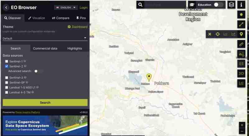
すべてのバンドのセンチネル画像をダウンロードするには:

• アカウントを作成する必要があります
• 自分のエリアで画像を見つけて、興味のあるエリアをカバーするグリッドを選択します
• グリッドにズームし、右の垂直バーの アイコンをクリックします
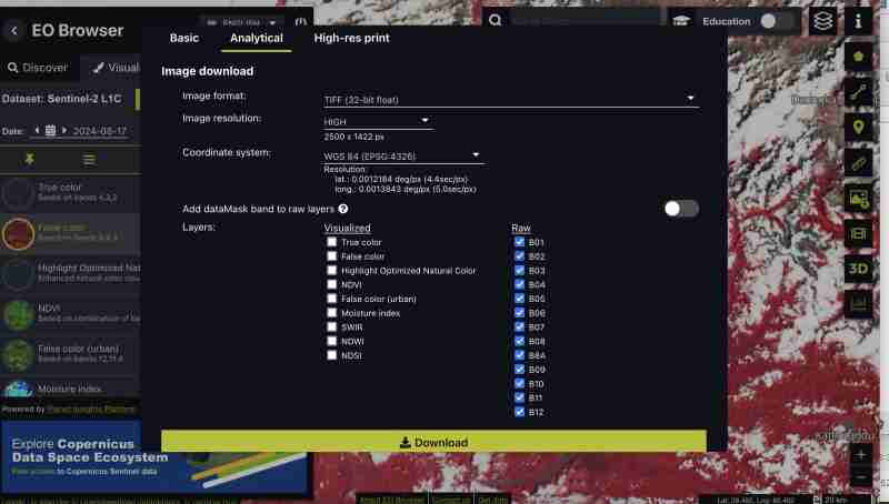
• その後、分析タブに移動し、画像形式が tiff 32 ビット、高解像度、wgs1984 形式ですべてのバンドを選択し、すべてのバンドがチェックされています

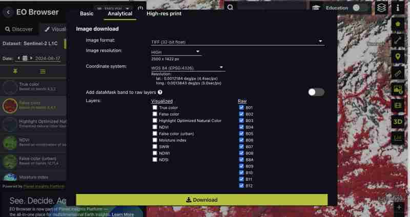
必要に応じて、NDVI、フォールスカラー tiff のみ、または特定のバンドなど、事前に生成されたインデックスをダウンロードすることもできます。自分で処理したいので、すべてのバンドをダウンロードしています

• ダウンロードをクリックします

前処理

生の形式をダウンロードしたため、すべてのバンドをセンチネルから別の tiff として取得します

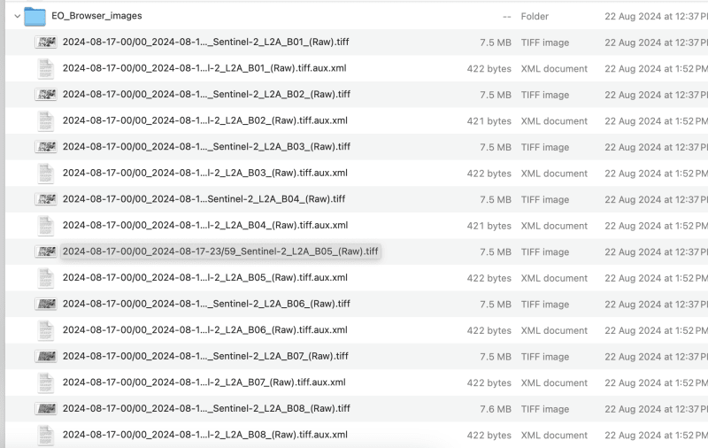
• 合成画像を作成しましょう:

これは GIS ツールまたは gdal を通じて実行できます

1. gdal_merge の使用:

ファイル名にスラッシュが含まれないように、ダウンロードしたファイルの名前を次のように Band1,band2 に変更する必要があります
この演習ではバンド 9 まで処理しましょう。必要に応じてバンドを選択できます

gdal_merge.py -separate -o sentinel2_composite.tif band1.tif band2.tif band3.tif band4.tif band5.tif band6.tif band7.tif band8.tif band9.tif 

1. QGIS の使用 :

• すべての個々のバンドを QGIS にロードします
• ラスターに移動 >その他＞マージ

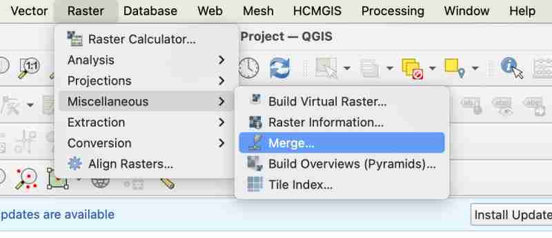
• マージ中に、「各入力ファイルを sep バンドに配置する」にチェックを入れる必要があります

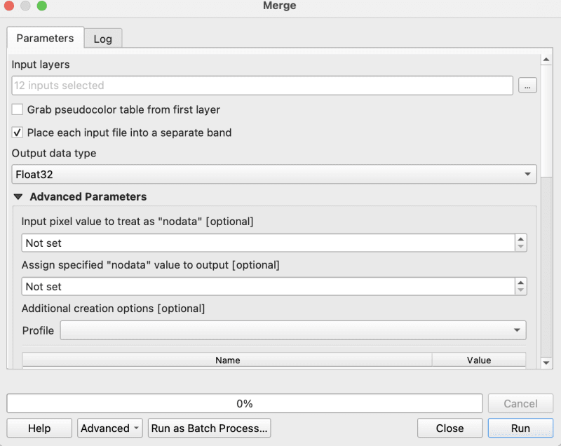
• 次に、マージされた tiff を複合として生の geotiff にエクスポートします

ハウスキーピング

• 画像が WGS1984 にあることを確認してください 私たちの場合、画像はすでに ws1984 にあるため、変換の必要はありません
• nodata がないことを確認し、ある場合は 0 を入力します。

  gdalwarp -overwrite -dstnodata 0 "$input_file" "${output_file}_nodata.tif"

• 最後に、出力イメージが COG であることを確認します。

  gdal_translate -of COG "$input_file" "$output_file"

これらを自動化するために、cog2h3 リポジトリで提供されている bash スクリプトを使用しています

sudo bash pre.sh sentinel2_composite.tif

h3 セルのプロセスと作成

前処理スクリプトが完了したので、いよいよ合成歯車画像の各バンドの h3 セルの計算に進みましょう

• cog2h3 をインストールする

  pip install cog2h3

• データベース認証情報をエクスポートします

  export DATABASE_URL="postgresql://user:password@host:port/database"

• 走る

このセンチネル画像には解像度 10 を使用していますが、h3 セルをラスター内の最小ピクセルよりも小さくする、ラスターに最適な解像度を印刷するスクリプト自体にも表示されます。

  cog2h3 --cog sentinel2_composite_preprocessed.tif --table sentinel --multiband --res 10

結果を計算して postgresql に保存するのに 1 分かかりました

ログ:

2024-08-24 08:39:43,233 - INFO - Starting processing
2024-08-24 08:39:43,234 - INFO - COG file already exists at sentinel2_composite_preprocessed.tif
2024-08-24 08:39:43,234 - INFO - Processing raster file: sentinel2_composite_preprocessed.tif
2024-08-24 08:39:43,864 - INFO - Determined Min fitting H3 resolution for band 1: 11
2024-08-24 08:39:43,865 - INFO - Resampling original raster to: 200.786148m
2024-08-24 08:39:44,037 - INFO - Resampling Done for band 1
2024-08-24 08:39:44,037 - INFO - New Native H3 resolution for band 1: 10
2024-08-24 08:39:44,738 - INFO - Calculation done for res:10 band:1
2024-08-24 08:39:44,749 - INFO - Determined Min fitting H3 resolution for band 2: 11
2024-08-24 08:39:44,749 - INFO - Resampling original raster to: 200.786148m
2024-08-24 08:39:44,757 - INFO - Resampling Done for band 2
2024-08-24 08:39:44,757 - INFO - New Native H3 resolution for band 2: 10
2024-08-24 08:39:45,359 - INFO - Calculation done for res:10 band:2
2024-08-24 08:39:45,366 - INFO - Determined Min fitting H3 resolution for band 3: 11
2024-08-24 08:39:45,366 - INFO - Resampling original raster to: 200.786148m
2024-08-24 08:39:45,374 - INFO - Resampling Done for band 3
2024-08-24 08:39:45,374 - INFO - New Native H3 resolution for band 3: 10
2024-08-24 08:39:45,986 - INFO - Calculation done for res:10 band:3
2024-08-24 08:39:45,994 - INFO - Determined Min fitting H3 resolution for band 4: 11
2024-08-24 08:39:45,994 - INFO - Resampling original raster to: 200.786148m
2024-08-24 08:39:46,003 - INFO - Resampling Done for band 4
2024-08-24 08:39:46,003 - INFO - New Native H3 resolution for band 4: 10
2024-08-24 08:39:46,605 - INFO - Calculation done for res:10 band:4
2024-08-24 08:39:46,612 - INFO - Determined Min fitting H3 resolution for band 5: 11
2024-08-24 08:39:46,612 - INFO - Resampling original raster to: 200.786148m
2024-08-24 08:39:46,619 - INFO - Resampling Done for band 5
2024-08-24 08:39:46,619 - INFO - New Native H3 resolution for band 5: 10
2024-08-24 08:39:47,223 - INFO - Calculation done for res:10 band:5
2024-08-24 08:39:47,230 - INFO - Determined Min fitting H3 resolution for band 6: 11
2024-08-24 08:39:47,230 - INFO - Resampling original raster to: 200.786148m
2024-08-24 08:39:47,239 - INFO - Resampling Done for band 6
2024-08-24 08:39:47,239 - INFO - New Native H3 resolution for band 6: 10
2024-08-24 08:39:47,829 - INFO - Calculation done for res:10 band:6
2024-08-24 08:39:47,837 - INFO - Determined Min fitting H3 resolution for band 7: 11
2024-08-24 08:39:47,837 - INFO - Resampling original raster to: 200.786148m
2024-08-24 08:39:47,845 - INFO - Resampling Done for band 7
2024-08-24 08:39:47,845 - INFO - New Native H3 resolution for band 7: 10
2024-08-24 08:39:48,445 - INFO - Calculation done for res:10 band:7
2024-08-24 08:39:48,453 - INFO - Determined Min fitting H3 resolution for band 8: 11
2024-08-24 08:39:48,453 - INFO - Resampling original raster to: 200.786148m
2024-08-24 08:39:48,461 - INFO - Resampling Done for band 8
2024-08-24 08:39:48,461 - INFO - New Native H3 resolution for band 8: 10
2024-08-24 08:39:49,046 - INFO - Calculation done for res:10 band:8
2024-08-24 08:39:49,054 - INFO - Determined Min fitting H3 resolution for band 9: 11
2024-08-24 08:39:49,054 - INFO - Resampling original raster to: 200.786148m
2024-08-24 08:39:49,062 - INFO - Resampling Done for band 9
2024-08-24 08:39:49,063 - INFO - New Native H3 resolution for band 9: 10
2024-08-24 08:39:49,647 - INFO - Calculation done for res:10 band:9
2024-08-24 08:39:51,435 - INFO - Converting H3 indices to hex strings
2024-08-24 08:39:51,906 - INFO - Overall raster calculation done in 8 seconds
2024-08-24 08:39:51,906 - INFO - Creating or replacing table sentinel in database
2024-08-24 08:40:03,153 - INFO - Table sentinel created or updated successfully in 11.25 seconds.
2024-08-24 08:40:03,360 - INFO - Processing completed

分析する

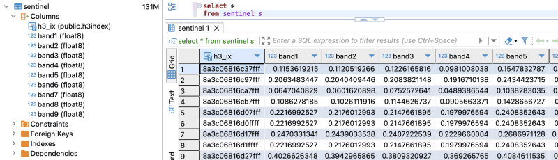
postgresql にデータがあるので、分析してみましょう

• 処理したすべてのバンドがあることを確認します (バンド 1 から 9 まで処理したことを思い出してください)

select *
from sentinel

• 各セルの ndvi を計算する

explain analyze 
select h3_ix , (band8-band4)/(band8+band4) as ndvi
from public.sentinel

クエリプラン:

QUERY PLAN                                                                                                       |
-----------------------------------------------------------------------------------------------------------------+
Seq Scan on sentinel  (cost=0.00..28475.41 rows=923509 width=16) (actual time=0.014..155.049 rows=923509 loops=1)|
Planning Time: 0.080 ms                                                                                          |
Execution Time: 183.764 ms                                                                                       |

As you can see here for all the rows in that area the calculation is instant . This is true for all other indices and you can compute complex indices join with other tables using the h3_ix primary key and derive meaningful result out of it without worrying as postgresql is capable of handling complex queries and table join.

Visualize and verification

Lets visualize and verify if the computed indices are true

• Create table ( for visualizing in QGIS )

create table ndvi_sentinel
as(
select h3_ix , (band8-band4)/(band8+band4) as ndvi
from public.sentinel )

• Lets add geometry to visualize the h3 cells This is only necessary to visualize in QGIS , if you build an minimal API by yourself you don't need this as you can construct geometry directly from query

ALTER TABLE ndvi_sentinel  
ADD COLUMN geometry geometry(Polygon, 4326) 
GENERATED ALWAYS AS (h3_cell_to_boundary_geometry(h3_ix)) STORED;

• Create index on geometry

create index on ndvi_sentinel(geometry);

• Connect your database in QGIS and visualize the table on the basis of ndvi value Lets get the area near Fewa lake or cloud

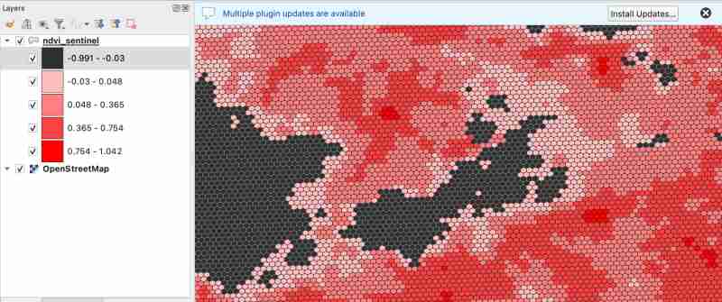
As we know value between -1.0 to 0.1 should represent Deep water or dense clouds
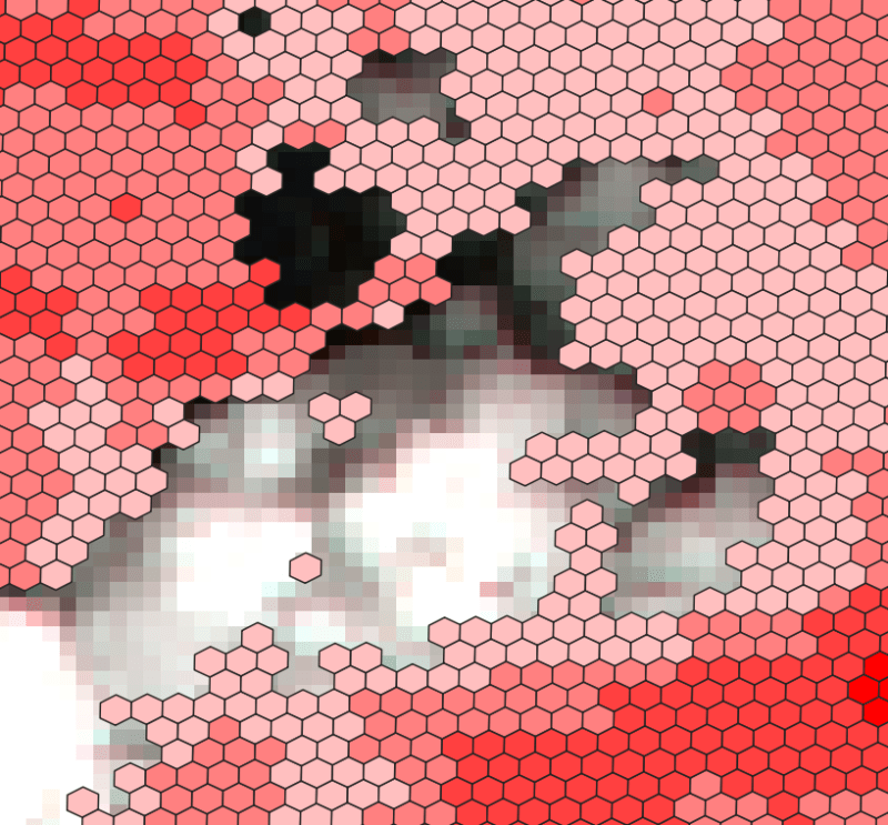
lets see if thats true ( making first category as transparent to see the underlying image )

• Check clouds :

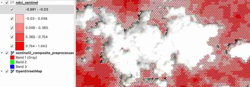
• Check Lake

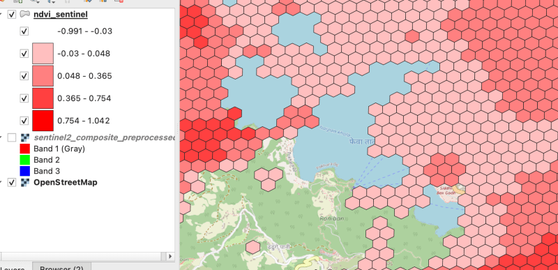
As there were clouds around the lake hence nearby fields are covered by cloud which makes sense

Thank you for reading ! See you in next blog

以上がマルチバンド ラスターを処理 (Sentinel-hndex を使用してインデックスを作成)の詳細内容です。詳細については、PHP 中国語 Web サイトの他の関連記事を参照してください。