Guide de l'indexation spatiale Uber & # 039;

In today’s data-driven world, efficient geospatial indexing is crucial for applications ranging from ride-sharing and logistics to environmental monitoring and disaster response. Uber’s H3, a powerful open-source spatial indexing system, provides a unique hexagonal grid-based solution that enables seamless geospatial analysis and fast query execution. Unlike traditional rectangular grid systems, H3’s hierarchical hexagonal tiling ensures uniform spatial coverage, better adjacency properties, and reduced distortion. This guide explores H3’s core concepts, installation, functionality, use cases, and best practices to help developers and data scientists leverage its full potential.

Learning Objectives

• Understand the fundamentals of Uber’s H3 spatial indexing system and its advantages over traditional grid systems.
• Learn how to install and set up H3 for geospatial applications in Python, JavaScript, and other languages.
• Explore H3’s hierarchical hexagonal grid structure and its benefits for spatial accuracy and indexing.
• Gain hands-on experience with core H3 functions like neighbor lookup, polygon indexing, and distance calculations.
• Discover real-world applications of H3, including machine learning, disaster response, and environmental monitoring.

This article was published as a part of the Data Science Blogathon.

Table of contents

• What is Uber H3?
• What is Spatial Indexing?
• Installation Guide (Python, JavaScript, Go, C, etc.)
• Data Structure and Hierarchical Indexing
• Core Functions
• Use Cases
• Combining H3 with Machine Learning
• Disaster Response and Environmental Monitoring
• Strengths and Weaknesses of H3
• Conclusion
• Frequently Asked Questions

What is Uber H3?

Uber H3 is an open-source, hexagonal hierarchical spatial indexing system developed by Uber. It is designed to efficiently partition and index geographic space, enabling advanced geospatial analysis, fast queries, and seamless visualization. Unlike traditional grid systems that use square or rectangular tiles, H3 utilizes hexagons, which provide superior spatial relationships, better adjacency properties, and minimize distortion when representing the Earth’s surface.

Why Uber Developed H3?

Uber developed H3 to solve key challenges in geospatial computing, particularly in ride-sharing, logistics, and location-based services. Traditional approaches based on latitude-longitude coordinates, rectangular grids, or QuadTrees often suffer from inconsistencies in resolution, inefficient spatial queries, and poor representation of real-world spatial relationships. H3 addresses these limitations by:

• Providing a uniform, hierarchical hexagonal grid that allows for seamless scalability across different resolutions.
• Enabling fast nearest-neighbour lookups and efficient spatial indexing for ride-demand forecasting, routing, and supply distribution.
• Supporting spatial queries and geospatial clustering with high accuracy and minimal computational overhead.

Today, H3 is widely used in applications beyond Uber, including environmental monitoring, geospatial analytics, and geographic information systems (GIS).

What is Spatial Indexing?

Spatial indexing is a technique used to structure and organize geospatial data efficiently, allowing for fast spatial queries and improved data retrieval performance. It is crucial for tasks such as:

• Nearest neighbor search
• Geospatial clustering
• Efficient geospatial joins
• Region-based filtering

H3 enhances spatial indexing by using a hexagonal grid system, which improves spatial accuracy, provides better adjacency properties, and reduces distortions found in traditional grid-based systems.

Installation Guide (Python, JavaScript, Go, C, etc.)

Setting Up H3 in a Development Environment

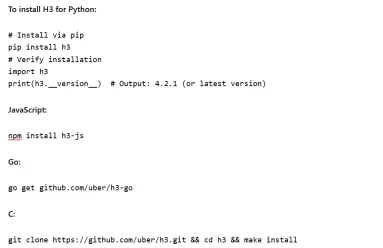
Let us now set up H3 in a development environment below:

# Create a virtual environment
python -m venv h3_env
source h3_env/bin/activate  # Linux/macOS
h3_env\Scripts\activate      # Windows

# Install dependencies
pip install h3 geopandas matplotlib

Data Structure and Hierarchical Indexing

Below we will understand data structure and hierarchical indexing in detail:

Hexagonal Grid System

H3’s hexagonal grid partitions Earth into 122 base cells (resolution 0), comprising 110 hexagons and 12 pentagons to approximate spherical geometry.Each cell undergoes hierarchical subdivision usingaperture 7partitioning, where every parent hexagon contains 7 child cells at the next resolution level.This creates 16 resolution levels (0-15) with exponentially decreasing cell sizes:

Resolution	Avg Edge Length (km)	Avg Area (km²)	Cell Count per Parent
0	1,107.712	4,250,546	–
5	8.544	252.903	16,807
9	0.174	0.105	40,353,607
15	0.0005	0.0000009	7^15 ≈ 4.7e12

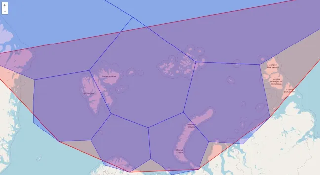
The code below demonstrates H3’s hierarchical hexagonal grid system :

import folium
import h3

base_cell = '8001fffffffffff'  # Resolution 0 pentagon
children = h3.cell_to_children(base_cell, res=1)

# Create a map centered at the center of the base hexagon
base_center = h3.cell_to_latlng(base_cell)
GeoSpatialMap = folium.Map(location=[base_center[0], base_center[1]], zoom_start=9)

# Function to get hexagon boundaries
def get_hexagon_bounds(h3_address):
    boundaries = h3.cell_to_boundary(h3_address)
    # Folium expects coordinates in [lat, lon] format
    return [[lat, lng] for lat, lng in boundaries]

# Add base hexagon
folium.Polygon(
    locations=get_hexagon_bounds(base_cell),
    color='red',
    fill=True,
    weight=2,
    popup=f'Base: {base_cell}'
).add_to(GeoSpatialMap)

# Add children hexagons
for child in children:
    folium.Polygon(
        locations=get_hexagon_bounds(child),
        color='blue',
        fill=True,
        weight=1,
        popup=f'Child: {child}'
    ).add_to(GeoSpatialMap)

GeoSpatialMap

Resolution Levels and Hierarchical Indexing

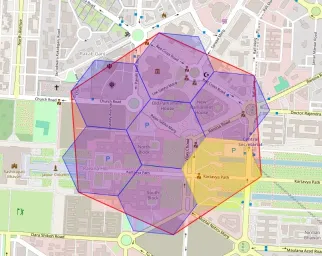
The hierarchical indexing structure enables multi-resolution analysis through parent-child relationships.H3 supports hierarchical resolution levels (from 0 to 15), allowing data to be indexed at different granularities.

The given code below shows this relationship:

delhi_cell = h3.latlng_to_cell(28.6139, 77.2090, 9)  # New Delhi coordinates

# Traverse hierarchy upwards
parent = h3.cell_to_parent(delhi_cell, res=8)
print(f"Parent at res 8: {parent}")

# Traverse hierarchy downwards
children = h3.cell_to_children(parent, res=9)
print(f"Contains {len(children)} children")

# Create a new map centered on New Delhi
delhi_map = folium.Map(location=[28.6139, 77.2090], zoom_start=15)

# Add the parent hexagon (resolution 8)
folium.Polygon(
    locations=get_hexagon_bounds(parent),
    color='red',
    fill=True,
    weight=2,
    popup=f'Parent: {parent}'
).add_to(delhi_map)

# Add all children hexagons (resolution 9)
for child_cell in children:
    color = 'yellow' if child_cell == delhi_cell else 'blue'
    folium.Polygon(
        locations=get_hexagon_bounds(child_cell),
        color=color,
        fill=True,
        weight=1,
        popup=f'Child: {child_cell}'
    ).add_to(delhi_map)

delhi_map

H3 Index Encoding

The H3 index encodes geospatial data into a64-bit unsigned integer(commonly represented as a 15-character hexadecimal string like‘89283082837ffff’). H3 indexes have the following architecture:

4 bits	3 bits	7 bits	45 bits
Mode and Resolution	Reserved	Base Cell	Child digits

We can understand the encoding process by the following code below:

import h3

# Convert coordinates to H3 index (resolution 9)

lat, lng = 37.7749, -122.4194  # San Francisco
h3_index = h3.latlng_to_cell(lat, lng, 9)
print(h3_index)  # '89283082803ffff'

# Deconstruct index components
## Get the resolution

resolution = h3.get_resolution(h3_index)
print(f"Resolution: {resolution}")

# Output: 9

# Get the base cell number
base_cell = h3.get_base_cell_number(h3_index)
print(f"Base cell: {base_cell}")
# Output: 20

# Check if its a pentagon
is_pentagon = h3.is_pentagon(h3_index)
print(f"Is pentagon: {is_pentagon}")
# Output: False

# Get the icosahedron face
face = h3.get_icosahedron_faces(h3_index)
print(f"Face number: {face}")
# Output: [7]

# Get the child cells
child_cells = h3.cell_to_children(h3.cell_to_parent(h3_index, 8), 9)
print(f"child cells: {child_cells}")
# Output: ['89283082803ffff', '89283082807ffff', '8928308280bffff', '8928308280fffff', 
#          '89283082813ffff', '89283082817ffff', '8928308281bffff']

Core Functions

Apart from the Hierarchical Indexing, some of the other Core functions of H3 are as follows:

• Neighbor Lookup & Traversal
• Polygon to H3 Indexing
• H3 Grid Distance and K-Ring

Neighbor Lookup andTraversal

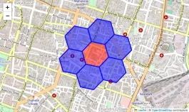
Neighbor lookup traversal refers toidentifying and navigating between adjacent cellsin Uber’s H3 hexagonal grid system. This enables spatial queries like “find all cells within a radius ofksteps” from a target cell. This concept can be understood from the code below:

import h3

# Define latitude, longitude for Kolkata
lat, lng = 22.5744, 88.3629
resolution = 9
h3_index = h3.latlng_to_cell(lat, lng, resolution)
print(h3_index)  # e.g., '89283082837ffff'

# Find all neighbors within 1 grid step
neighbors = h3.grid_disk(h3_index, k=1)
print(len(neighbors))  # 7 (6 neighbors + the original cell)

# Check edge adjacency
is_neighbor = h3.are_neighbor_cells(h3_index, neighbors[0])
print(is_neighbor)  # True or False

To generate the visualization of this we can simply use the code given below:

import h3
import folium

# Define latitude, longitude for Kolkata
lat, lng = 22.5744, 88.3629
resolution = 9  # H3 resolution

# Convert lat/lng to H3 index
h3_index = h3.latlng_to_cell(lat, lng, resolution)

# Get neighboring hexagons
neighbors = h3.grid_disk(h3_index, k=1)

# Initialize map centered at the given location
m = folium.Map(location=[lat, lng], zoom_start=12)

# Function to add hexagons to the map
def add_hexagon(h3_index, color):
    """ Adds an H3 hexagon to the folium map """
    boundary = h3.cell_to_boundary(h3_index)
    # Convert to [lat, lng] format for folium
    boundary = [[lat, lng] for lat, lng in boundary]
    folium.Polygon(
        locations=boundary,
        color=color,
        fill=True,
        fill_color=color,
        fill_opacity=0.5
    ).add_to(m)

# Add central hexagon in red
add_hexagon(h3_index, "red")

# Add neighbor hexagons in blue
for neighbor in neighbors:
    if neighbor != h3_index:  # Avoid recoloring the center
        add_hexagon(neighbor, "blue")

# Display the map
m

Use cases of Neighbor Lookup & Traversal are as follows:

• Ride Sharing: Find available drivers within a 5-minute drive radius.
• Spatial Aggregation: Calculate total rainfall in cells within 10 km of a flood zone.
• Machine Learning: Generate neighborhood features for demand prediction models.

Polygon to H3 Indexing

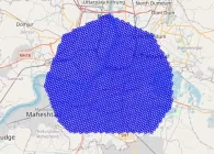
Converting a polygon to H3 indexes involves identifying all hexagonal cells at a specified resolution thatfully or partially intersectwith the polygon. This is critical for spatial operations like aggregating data within geographic boundaries. This could be understood from the given code below:

import h3   

# Define a polygon (e.g., San Francisco bounding box)  
polygon_coords = h3.LatLngPoly(
    [(37.708, -122.507), (37.708, -122.358), (37.832, -122.358), (37.832, -122.507)]
)

# Convert polygon to H3 cells (resolution 9)  
resolution = 9  
cells = h3.polygon_to_cells(polygon_coords, res=resolution)  
print(f"Total cells: {len(cells)}")  
# Output: ~ 1651

To visualize this we can follow the given code below:

import h3
import folium
from h3 import LatLngPoly

# Define a bounding polygon for Kolkata
kolkata_coords = LatLngPoly([
    (22.4800, 88.2900),  # Southwest corner
    (22.4800, 88.4200),  # Southeast corner
    (22.5200, 88.4500),  # East
    (22.5700, 88.4500),  # Northeast
    (22.6200, 88.4200),  # North
    (22.6500, 88.3500),  # Northwest
    (22.6200, 88.2800),  # West
    (22.5500, 88.2500),  # Southwest
    (22.5000, 88.2700)   # Return to starting area
])
# Add more boundary coordinates for more specific map

# Convert polygon to H3 cells
resolution = 9
cells = h3.polygon_to_cells(kolkata_coords, res=resolution)

# Create a Folium map centered around Kolkata
kolkata_map = folium.Map(location=[22.55, 88.35], zoom_start=12)

# Add each H3 cell as a polygon
for cell in cells:
    boundaries = h3.cell_to_boundary(cell)
    # Convert to [lat, lng] format for folium
    boundaries = [[lat, lng] for lat, lng in boundaries]
    folium.Polygon(
        locations=boundaries,
        color='blue',
        weight=1,
        fill=True,
        fill_opacity=0.4,
        popup=cell
    ).add_to(kolkata_map)

# Show map
kolkata_map

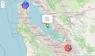
H3 Grid Distance and K-Ring

Grid distancemeasures the minimum number of steps required to traverse from one H3 cell to another, moving through adjacent cells. Unlike geographical distance, it’s a topological metric based on hexagonal grid connectivity. And we should keep in mind that higher resolutions yield smaller steps so the grid distance would be larger.

import h3
from h3 import latlng_to_cell

# Define two H3 cells at resolution 9  
cell_a = latlng_to_cell(37.7749, -122.4194, 9)  # San Francisco  
cell_b = latlng_to_cell(37.3382, -121.8863, 9)  # San Jose  

# Calculate grid distance  
distance = h3.grid_distance(cell_a, cell_b)  
print(f"Grid distance: {distance} steps")  
# Output: Grid distance: 220 steps (approx)

We can visualize this with the following given code:

import h3
import folium
from h3 import latlng_to_cell
from shapely.geometry import Polygon

# Function to get H3 polygon boundary
def get_h3_polygon(h3_index):
    boundary = h3.cell_to_boundary(h3_index)
    return [(lat, lon) for lat, lon in boundary]

# Define two H3 cells at resolution 6
cell_a = latlng_to_cell(37.7749, -122.4194, 6)  # San Francisco
cell_b = latlng_to_cell(37.3382, -121.8863, 6)  # San Jose

# Get hexagon boundaries
polygon_a = get_h3_polygon(cell_a)
polygon_b = get_h3_polygon(cell_b)

# Compute grid distance
distance = h3.grid_distance(cell_a, cell_b)

# Create a folium map centered between the two locations
map_center = [(37.7749 + 37.3382) / 2, (-122.4194 + -121.8863) / 2]
m = folium.Map(location=map_center, zoom_start=9)

# Add H3 hexagons to the map
folium.Polygon(locations=polygon_a, color='blue', fill=True, fill_opacity=0.4, popup="San Francisco (H3)").add_to(m)
folium.Polygon(locations=polygon_b, color='red', fill=True, fill_opacity=0.4, popup="San Jose (H3)").add_to(m)

# Add markers for the center points
folium.Marker([37.7749, -122.4194], popup="San Francisco").add_to(m)
folium.Marker([37.3382, -121.8863], popup="San Jose").add_to(m)

# Display distance
folium.Marker(map_center, popup=f"H3 Grid Distance: {distance} steps", icon=folium.Icon(color='green')).add_to(m)

# Show the map
m

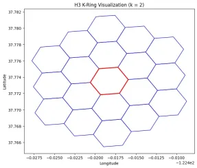
AndK-Ring(orgrid disk) in H3 refers to all hexagonal cells withinkgrid stepsfrom a central cell. This includes:

• The central cell itself (at step 0).
• Immediate neighbors (step 1).
• Cells at progressively larger distances up to `k` steps.

import h3  

# Define a central cell (San Francisco at resolution 9)  
central_cell = h3.latlng_to_cell(37.7749, -122.4194, 9)  
k = 2  

# Generate K-Ring (cells within 2 steps)  
k_ring = h3.grid_disk(central_cell, k)  
print(f"Total cells: {len(k_ring)}")  # e.g., 19 cells  

This can be visualized from the plot given below:

import h3
import matplotlib.pyplot as plt
from shapely.geometry import Polygon
import geopandas as gpd

# Define central point (latitude, longitude) for San Francisco [1]
lat, lng = 37.7749, -122.4194
resolution = 9  # Choose resolution (e.g., 9) [1]

# Obtain central H3 cell index for the given point [1]
center_h3 = h3.latlng_to_cell(lat, lng, resolution)
print("Central H3 cell:", center_h3)  # Example output: '89283082837ffff'

# Define k value (number of grid steps) for the k-ring [1]
k = 2

# Generate k-ring of cells: all cells within k grid steps of centerH3 [1]
k_ring_cells = h3.grid_disk(center_h3, k)
print("Total k-ring cells:", len(k_ring_cells))
# For a standard hexagon (non-pentagon), k=2 typically returns 19 cells:
# 1 (central cell) + 6 (neighbors at distance 1) + 12 (neighbors at distance 2)

# Convert each H3 cell into a Shapely polygon for visualization [1][6]
polygons = []
for cell in k_ring_cells:
    # Get the cell boundary as a list of (lat, lng) pairs; geo_json=True returns in [lat, lng]
    boundary = h3.cell_to_boundary(cell)
    # Swap to (lng, lat) because Shapely expects (x, y)
    poly = Polygon([(lng, lat) for lat, lng in boundary])
    polygons.append(poly)

# Create a GeoDataFrame for plotting the hexagonal cells [2]
gdf = gpd.GeoDataFrame({'h3_index': list(k_ring_cells)}, geometry=polygons)

# Plot the boundaries of the k-ring cells using Matplotlib [2][6]
fig, ax = plt.subplots(figsize=(8, 8))
gdf.boundary.plot(ax=ax, color='blue', lw=1)

# Highlight the central cell by plotting its boundary in red [1]
central_boundary = h3.cell_to_boundary(center_h3)
central_poly = Polygon([(lng, lat) for lat, lng in central_boundary])
gpd.GeoSeries([central_poly]).boundary.plot(ax=ax, color='red', lw=2)

# Set plot labels and title for clear visualization
ax.set_title("H3 K-Ring Visualization (k = 2)")
ax.set_xlabel("Longitude")
ax.set_ylabel("Latitude")
plt.show()

Use Cases

While the use cases of H3 are only limited to one’s creativity, here are few examples of it :

Efficient Geo-Spatial Queries

H3 excels at optimizing location-based queries, such as counting points of interest (POIs) within dynamic geographic boundaries.

In this use case, we demonstrate how H3 can be applied to analyze and visualize ride pickup density in San Francisco using Python. To simulate real-world ride data, we generate random GPS coordinates centered around San Francisco. We also assign each ride a random timestamp within the past week to create a realistic dataset. Each ride’s latitude and longitude are converted into an H3 index at resolution 10, a fine-grained hexagonal grid that helps in spatial aggregation. To analyze local ride pickup density, we select a target H3 cell and retrieve all nearby cells within two hexagonal rings using h3.grid_disk. To visualize the spatial distribution of pickups, we overlay the H3 hexagons onto a Folium map.

Code Implementation

The execution code is given below:

import pandas as pd
import h3
import folium
import matplotlib.pyplot as plt
import numpy as np
from datetime import datetime, timedelta
import random

# Create sample GPS data around San Francisco
# Center coordinates for San Francisco
center_lat, center_lng = 37.7749, -122.4194

# Generate synthetic ride data
num_rides = 1000
np.random.seed(42)  # For reproducibility

# Generate random coordinates around San Francisco
lats = np.random.normal(center_lat, 0.02, num_rides)  # Normal distribution around center
lngs = np.random.normal(center_lng, 0.02, num_rides)

# Generate timestamps for the past week
start_time = datetime.now() - timedelta(days=7)
timestamps = [start_time + timedelta(minutes=random.randint(0, 10080)) for _ in range(num_rides)]
timestamp_strs = [ts.strftime('%Y-%m-%d %H:%M:%S') for ts in timestamps]

# Create DataFrame
rides = pd.DataFrame({
    'lat': lats,
    'lng': lngs,
    'timestamp': timestamp_strs
})

# Convert coordinates to H3 indexes (resolution 10)
rides["h3"] = rides.apply(
    lambda row: h3.latlng_to_cell(row["lat"], row["lng"], 10), axis=1  
)

# Count pickups per cell
pickup_counts = rides["h3"].value_counts().reset_index()
pickup_counts.columns = ["h3", "counts"]

# Query pickups within a specific cell and its neighbors 
target_cell = h3.latlng_to_cell(37.7749, -122.4194, 10)
neighbors = h3.grid_disk(target_cell, k=2)
local_pickups = pickup_counts[pickup_counts["h3"].isin(neighbors)]

# Visualize the spatial query results
map_center = h3.cell_to_latlng(target_cell)
m = folium.Map(location=map_center, zoom_start=15)

# Function to get hexagon boundaries
def get_hexagon_bounds(h3_address):
    boundaries = h3.cell_to_boundary(h3_address)
    return [[lat, lng] for lat, lng in boundaries]

# Add target cell
folium.Polygon(
    locations=get_hexagon_bounds(target_cell),
    color='red',
    fill=True,
    weight=2,
    popup=f'Target Cell: {target_cell}'
).add_to(m)

# Color scale for counts
max_count = local_pickups["counts"].max()
min_count = local_pickups["counts"].min()

# Add neighbor cells with color intensity based on pickup counts
for _, row in local_pickups.iterrows():
    if row["h3"] != target_cell:
        # Calculate color intensity based on count
        intensity = (row["counts"] - min_count) / (max_count - min_count) if max_count > min_count else 0.5
        color = f'#{int(255*(1-intensity)):02x}{int(200*(1-intensity)):02x}ff'
        
        folium.Polygon(
            locations=get_hexagon_bounds(row["h3"]),
            color=color,
            fill=True,
            fill_opacity=0.7,
            weight=1,
            popup=f'Cell: {row["h3"]}<br>Pickups: {row["counts"]}'
        ).add_to(m)

# Create a heatmap visualization with matplotlib
plt.figure(figsize=(12, 8))
plt.title("H3 Grid Heatmap of Ride Pickups")

# Create a scatter plot for cells, size based on pickup counts
for idx, row in local_pickups.iterrows():
    center = h3.cell_to_latlng(row["h3"])
    plt.scatter(center[1], center[0], s=row["counts"]/2, 
                c=row["counts"], cmap='viridis', alpha=0.7)

plt.colorbar(label='Number of Pickups')
plt.xlabel('Longitude')
plt.ylabel('Latitude')
plt.grid(True)

# Display both visualizations
m  # Display the folium map

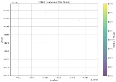
The above example highlights how H3 can be leveraged for spatial analysis in urban mobility. By converting raw GPS coordinates into a hexagonal grid, we can efficiently analyze ride density, detect hotspots, and visualize data in an insightful manner. H3’s flexibility in handling different resolutions makes it a valuable tool for geospatial analytics in ride-sharing, logistics, and urban planning applications.

Combining H3 with Machine Learning

H3 has been combined with Machine Learning to solve many real world problems. Uber reduced ETA prediction errors by 22% using H3-based ML models while Toulouse, France, used H3 + ML to optimize bike lane placement, increasing ridership by 18%.

In this use case, we demonstrate how H3 can be applied to analyze and predict traffic congestion in San Francisco using historical GPS ride data and machine learning techniques.To simulate real-world traffic conditions, we generate random GPS coordinates centered around San Francisco. Each ride is assigned a random timestamp within the past week, along with a randomly generated speed value.Each ride’s latitude and longitude are converted into an H3 index at resolution 10, enabling spatial aggregation and analysis.We extract features from a sample cell and its neighboring cells within two hexagonal rings to analyze local traffic conditions.To predict traffic congestion, we use an LSTM-based deep learning model. The model is designed to process historical traffic data and predict congestion probabilities.Using the trained model, we can predict the probability of congestion for a given cell.

Code Implementation

The execution code is given below :

import h3
import pandas as pd
import numpy as np
from datetime import datetime, timedelta
import random
import tensorflow as tf
from tensorflow.keras.layers import LSTM, Conv1D, Dense

# Create sample GPS data around San Francisco
center_lat, center_lng = 37.7749, -122.4194
num_rides = 1000
np.random.seed(42)  # For reproducibility

# Generate random coordinates around San Francisco
lats = np.random.normal(center_lat, 0.02, num_rides)
lngs = np.random.normal(center_lng, 0.02, num_rides)

# Generate timestamps for the past week
start_time = datetime.now() - timedelta(days=7)
timestamps = [start_time + timedelta(minutes=random.randint(0, 10080)) for _ in range(num_rides)]
timestamp_strs = [ts.strftime('%Y-%m-%d %H:%M:%S') for ts in timestamps]

# Generate random speed data
speeds = np.random.uniform(5, 60, num_rides)  # Speed in km/h

# Create DataFrame
gps_data = pd.DataFrame({
    'lat': lats,
    'lng': lngs,
    'timestamp': timestamp_strs,
    'speed': speeds
})

# Convert coordinates to H3 indexes (resolution 10)
gps_data["h3"] = gps_data.apply(
    lambda row: h3.latlng_to_cell(row["lat"], row["lng"], 10), axis=1
)

# Convert timestamp string to datetime objects
gps_data["timestamp"] = pd.to_datetime(gps_data["timestamp"])

# Aggregate speed and count per cell per 5-minute interval
agg_data = gps_data.groupby(["h3", pd.Grouper(key="timestamp", freq="5T")]).agg(
    avg_speed=("speed", "mean"),
    vehicle_count=("h3", "count")
).reset_index()

# Example: Use a cell from our existing dataset
sample_cell = gps_data["h3"].iloc[0]
neighbors = h3.grid_disk(sample_cell, 2)

def get_kring_features(cell, k=2):
    neighbors = h3.grid_disk(cell, k)
    return {f"neighbor_{i}": neighbor for i, neighbor in enumerate(neighbors)}

# Placeholder function for feature extraction
def fetch_features(neighbors, agg_data):
    # In a real implementation, this would fetch historical data for the neighbors
    # This is just a simplified example that returns random data
    return np.random.rand(1, 6, len(neighbors))  # 1 sample, 6 timesteps, features per neighbor

# Define a skeleton model architecture
def create_model(input_shape):
    model = tf.keras.Sequential([
        LSTM(64, return_sequences=True, input_shape=input_shape),
        LSTM(32),
        Dense(16, activation='relu'),
        Dense(1, activation='sigmoid')
    ])
    model.compile(optimizer='adam', loss='binary_crossentropy', metrics=['accuracy'])
    return model

# Prediction function (would use a trained model in practice)
def predict_congestion(cell, model, agg_data):
    # Fetch neighbor cells
    neighbors = h3.grid_disk(cell, k=2)
    # Get historical data for neighbors
    features = fetch_features(neighbors, agg_data)
    # Predict
    return model.predict(features)[0][0]

# Create a skeleton model (not trained)
input_shape = (6, 19)  # 6 time steps, 19 features (for k=2 neighbors)
model = create_model(input_shape)

# Print information about what would happen in a real prediction
print(f"Sample cell: {sample_cell}")
print(f"Number of neighboring cells (k=2): {len(neighbors)}")
print("Model summary:")
model.summary()

# In practice, you would train the model before using it for predictions
# This would just show what a prediction call would look like:
congestion_prob = predict_congestion(sample_cell, model, agg_data)
print(f"Congestion probability: {congestion_prob:.2%}")

# example output- Congestion Probability: 49.09%

This example demonstrates how H3 can be leveraged for spatial analysis and traffic prediction. By converting GPS data into hexagonal grids, we can efficiently analyze traffic patterns, extract meaningful insights from neighboring regions, and use deep learning to predict congestion in real time. This approach can be applied to smart city planning, ride-sharing optimizations, and intelligent traffic management systems.

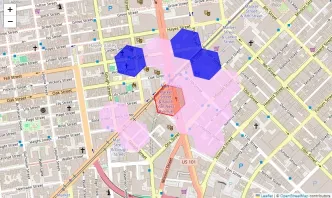
Disaster Response and Environmental Monitoring

Flood events representone of the mostcommon natural disasters requiring immediate response and resource allocation. H3 can significantly improve flood response efforts by integrating various data sources including flood zone maps, population density, building infrastructure, andreal-time water level readings.

The following Python implementation demonstrates howto use H3 for flood risk analysis byintegrating flooded area datawith building infrastructure information:

import h3
import folium
import pandas as pd
import numpy as np
from folium.plugins import MarkerCluster

# Create sample buildings dataset
np.random.seed(42)
num_buildings = 50

# Create buildings around San Francisco
center_lat, center_lng = 37.7749, -122.4194
building_types = ['residential', 'commercial', 'hospital', 'school', 'government']
building_weights = [0.6, 0.2, 0.1, 0.07, 0.03]  # Probability weights

# Generate building data
buildings_df = pd.DataFrame({
    'lat': np.random.normal(center_lat, 0.005, num_buildings),
    'lng': np.random.normal(center_lng, 0.005, num_buildings),
    'type': np.random.choice(building_types, size=num_buildings, p=building_weights),
    'capacity': np.random.randint(10, 1000, num_buildings)
})

# Add H3 index at resolution 10
buildings_df['h3_index'] = buildings_df.apply(
    lambda row: h3.latlng_to_cell(row['lat'], row['lng'], 10),
    axis=1
)

# Create some flood cells (let's use some cells where buildings are located)
# Taking a few cells where buildings are located to simulate a flood zone
flood_cells = set(buildings_df['h3_index'].sample(10))

# Create a map centered at the average of our coordinates
center_lat = buildings_df['lat'].mean()
center_lng = buildings_df['lng'].mean()
flood_map = folium.Map(location=[center_lat, center_lng], zoom_start=16)

# Function to get hexagon boundaries for folium
def get_hexagon_bounds(h3_address):
    boundaries = h3.cell_to_boundary(h3_address)
    # Folium expects coordinates in [lat, lng] format
    return [[lat, lng] for lat, lng in boundaries]

# Add flood zone cells
for cell in flood_cells:
    folium.Polygon(
        locations=get_hexagon_bounds(cell),
        color='blue',
        fill=True,
        fill_opacity=0.4,
        weight=2,
        popup=f'Flood Cell: {cell}'
    ).add_to(flood_map)

# Add building markers
for idx, row in buildings_df.iterrows():
    # Set color based on if building is affected
    if row['h3_index'] in flood_cells:
        color = 'red'
        icon = 'warning' if row['type'] in ['hospital', 'school'] else 'info-sign'
        prefix = 'glyphicon'
    else:
        color = 'green'
        icon = 'home'
        prefix = 'glyphicon'
    
    # Create marker with popup showing building details
    folium.Marker(
        location=[row['lat'], row['lng']],
        popup=f"Building Type: {row['type']}<br>Capacity: {row['capacity']}",
        tooltip=f"{row['type']} (Capacity: {row['capacity']})",
        icon=folium.Icon(color=color, icon=icon, prefix=prefix)
    ).add_to(flood_map)

# Add a legend as an HTML element
legend_html = '''
<div>
     <b>Flood Impact Analysis</b> <br>
     <i></i> Flood Zone <br>
     <i></i> Safe Buildings <br>
     <i></i> Affected Buildings <br>
     <i></i> Critical Facilities <br>
</div>
'''
flood_map.get_root().html.add_child(folium.Element(legend_html))

# Display the map
flood_map

This code provides an efficient method for visualizing and analyzing flood impacts using H3 spatial indexing and Folium mapping. By integrating spatial data clustering and interactive visualization, it enhances disaster response planning and urban risk management strategies. This approach can be extended to other geospatial challenges, such as wildfire risk assessment or transportation planning.

Strengths and Weaknesses of H3

The following table provides a detailed analysis of H3’s advantages and limitations based on industry implementations and technical evaluations:

Aspect	Strengths	Weaknesses
Geometry Properties	Hexagonal cells provide uniform distance metrics with equidistant neighbors. Better approximation of circles than square/rectangular grids. Minimizes both area and shape distortion globally	Cannot completely divide Earth into hexagons, requires 12 pentagon cells that create irregular adjacency patterns. Not a true equal-area system, despite aiming for “roughly equal-ish” areas
Hierarchical Structure	Efficiently changes precision (resolution) levels as needed. Compact 64-bit addresses for all resolutions- Parent-child tree with no shared parents.	Hierarchical nesting between resolutions isn’t perfect. Tiny discontinuities (gaps/overlaps) can occur at adjacent scales.Problematic for use cases requiring exact containment (e.g., parcel data)
Performance	H3-centric approaches can be up to 90x less expensive than geometry-centric operations. Significantly enhances processing efficiency with large dataset.Fast calculations between predictable cells in grid system	Processing large areas at high resolutions requires significant computational resources.Trade-off between precision and performance – higher resolutions consume more resources.
Spatial Analysis	Multi-resolution analysis from neighborhood to regional scales. Standardized format for integrating heterogeneous data sources. Uniform adjacency relationships simplify neighborhood searches	Polygon coverage is approximate with potential gaps at boundaries. Precision limitations dependent on chosen resolution level.Special handling required for polygon intersections
Implementation	Simple API with built-in utilities (geofence polyfill, hexagon compaction, GeoJSON output)- Well-suited for parallelized execution. Cell IDs can be used as columns in standard SQL functions.	Handling pentagon cells requires specialized code. Adapting existing workflows to H3 can be complex. Data quality dependencies affect analysis accuracy
Applications	Optimized for: geospatial analytics, mobility analysis, logistics, delivery services, telecoms, insurance risk assessment, and environmental monitoring.	Less suitable for applications requiring exact boundary definitions. May not be optimal for specialized cartographic purposes. Can involve computational complexity for real-time applications with limited resources.

Conclusion

Uber’s H3 spatial indexing system is a powerful tool for geospatial analysis, offering a hexagonal grid structure that enables efficient spatial queries, multi-resolution analysis, and seamless integration with modern data workflows. Its strengths lie in its uniform geometry, hierarchical design, and ability to handle large-scale datasets with speed and precision. From ride-sharing optimization to disaster response and environmental monitoring, H3 has proven its versatility across industries.

However, like any technology, H3 has limitations, such as handling pentagon cells, approximating polygon boundaries, and computational demands at high resolutions. By understanding its strengths and weaknesses, developers can leverage H3 effectively for applications requiring scalable and accurate geospatial insights.

As geospatial technology evolves, H3’s open-source ecosystem will likely see further enhancements, including integration with machine learning models, real-time analytics, and 3D spatial indexing. H3 is not just a tool but a foundation for building smarter geospatial solutions in an increasingly data-driven world.

Frequently Asked Questions

Q1. Where can I learn more about using H3?

A. Visit the official H3 documentation or explore open-source examples on GitHub. Uber’s engineering blog also provides insights into real-world applications of H3.

Q2. Is H3 suitable for real-time applications?

A. Yes! With its fast indexing and neighbor lookup capabilities, H3 is highly efficient for real-time geospatial applications like live traffic monitoring or disaster response coordination.

Q3. Can I use H3 with machine learning models?

A. Yes! H3 is well-suited for machine learning applications. By converting raw GPS data into hexagonal features (e.g., traffic density per cell), you can integrate spatial patterns into predictive models like demand forecasting or congestion prediction.

Q4. What programming languages are supported by H3?

A. The core H3 library is written in C but has bindings for Python, JavaScript, Go, Java, and more. This makes it versatile for integration into various geospatial workflows.

Q5. How does H3 handle the entire globe with hexagons?

A. While it’s impossible to tile a sphere perfectly with hexagons, H3 introduces 12 pentagon cells at each resolution to close gaps. To minimize their impact on most datasets, the system strategically places these pentagons over oceans or less significant areas.

The media shown in this article is not owned by Analytics Vidhya and is used at the Author’s discretion.

Ce qui précède est le contenu détaillé de. pour plus d'informations, suivez d'autres articles connexes sur le site Web de PHP en chinois!