Hard core to solve Sora's physics bug! Four top universities in the United States jointly released: Install a physics engine for the video generator

Some bugs appeared after Sora was released. Users on the Internet discovered some problems. Although the model did not fully understand the physical world, when the puppy was walking, its two front legs would Interleaving issues occur, causing the game to appear unexpectedly.

The interaction of objects is very important for generating video realism, but currently, it is still very difficult to synthesize the dynamic behavior of real 3D objects in interaction.

Action Conditioned Dynamics is a field of research that requires the perception of physical material properties of objects and the prediction of 3D motion based on these properties (such as object stiffness).

Evaluating physical material properties remains a thorny and unsolved problem due to the lack of data support, as measuring physical material properties of real objects is extremely difficult.

Recently, MIT, Stanford University, Columbia University, and Cornell University jointly proposed a physics-based model, PhysDreamer, that uses object dynamics learned from video generation models to learn priors , empowering interactive dynamics learning for static 3D objects.

Paper link: https://arxiv.org/pdf/2404.13026.pdf

Project Home page: https://physdreamer.github.io/

By refining prior knowledge, PhysDreamer can realize the response of physical objects to new interactions, such as external forces or agent operations, and through The effectiveness of the method is demonstrated on different examples of elastic objects, and user studies are used to evaluate the realism of the synthesized interactions.

Formalization of the problem

Given a static object represented by a 3D Gaussian(where xp represents the position and αp represents the opacity , Σp represents the covariance matrix, cp represents the color of the particle), the ultimate goal is to estimate the physical material property field of the object to achieve real interactive motion synthesis.

The specific properties include mass m, Young's modulus E and Poisson's ratio ν. Young's modulus is used to measure the stiffness of the material and determines the movement trajectory of the object in response to external forces: relatively A high Young's modulus results in smaller deformation, stiffer and higher frequency motion.

Simulated motion of flowers under the same force but with different Young’s modulus

So the researchers formalized the problem as estimating the spatially varying Young's modulus field E(x) of the 3D object, and can use to query the Young's modulus of the particle for particle simulation.

As for other physical properties, the mass m_p of the particle can be pre-calculated as the product of the constant density (ρ) and the particle volume Vp; the particle volume can be calculated by dividing the "volume of the background unit" by It is estimated by "the number of particles contained in the unit"; the influence of Poisson's ratio νp on the motion of the object is negligible and can be assumed to be a constant.

Model Architecture

PhysDreamer can estimate the material field of a static 3D object. The key idea is to generate a credible video of the moving object and then optimize the material field E(x ) to match synthetic motion.

Given an object represented as a 3D Gaussian, first render it from some viewpoint (with background), then use an image-to-video generation model to generate a reference video of the object in motion, Differentiable material point methods (MPM, Material Point Methods) and differentiable rendering are then used to optimize the spatially varying material field and initial velocity field, aiming to minimize the difference between the rendered video and the reference video.

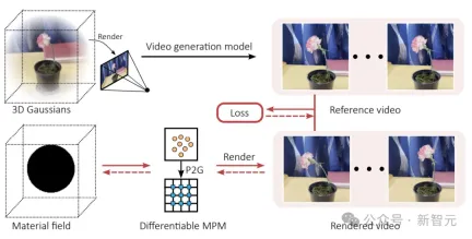
The dashed arrow represents the gradient flow

1. Basic knowledge

3D Gaussian uses a set of anisotropic 3D Gaussian kernels to represent the radiation field of the 3D scene. Although it is mainly introduced as a 3D new view synthesis method, due to the Lagrangian properties of 3D Gaussian, So it can be directly applied to particle physics simulators.

Similar to the PhysGaussian method, researchers use material point methods (MPM, Material Point Methods) to directly simulate object dynamics on Gaussian particles.

Since the 3D Gaussian distribution is mainly located on the surface of the object, an optional internal filling process can be applied to improve the realism of the simulation.

Continuum mechanics and elastic materials

In continuum mechanics, the deformation of the material is Simulation is carried out through a mapping function ϕ, which can convert the space point X of the material in the undeformed state into the point #In order to measure the local rotation and strain (strain) in material deformation, the concept of deformation gradient (deformation gradient) is introduced, which is the Jacobian matrix F of the mapping function ϕ, that is,

Deformation gradient is the key to understanding and describing the material stress-strain relationship, which involves the local deformation state of the material.

In highly elastic materials, the calculation of Cauchy stress (stress) relies on the strain energy density function ψ(F), which can quantify the degree of non-rigid deformation of the material; generally speaking , a function designed by materials scientists based on the principles of symmetry and rotational invariance of materials and matched to experimental data.

In addition, the energy density function in the fixed rotation hyperelastic model can be expressed by a singular value σi of the deformation gradient, and the model parameters μ and λ are related to the Young’s modulus E of the material Directly related to Poisson's ratio ν, these parameters are critical to understanding how materials behave when stressed.

##Material Point Method (MPM)

The researchers used the moving least squares material point method (MLS-MPM) to solve the governing equations of "elastic material dynamics", where ρ represents the density and v(x, t) represents the velocity field in the world space. , f represents external force.

MPM is a calculation method for simulating the dynamics of various materials, which combines the advantages of Euler and Lagrangian methods. It is particularly suitable for simulating the dynamic behavior of materials such as solids, fluids, sand, and cloth. It can effectively handle topological changes in materials, and can be easily parallelized on a graphics processing unit (GPU).

Spatial discretization is performed by treating the object as a series of Gaussian particles. Each particle p represents a small part of the volume of the object and carries volume, mass, position, velocity, deformation Properties such as gradient and local velocity field gradient.

The calculation process of MPM includes particle-to-grid (P2G) and grid-to-particle (G2P) transfer loops:

In the P2G stage, momentum is transferred from the particle to the grid, updating the velocity on the grid, and then these updated velocity information is passed back to the particle to update the particle's position and velocity. At the same time, the particle's local velocity gradient and The deformation gradient is also updated to reflect the current state of the material.

The MPM method can accurately simulate the complex dynamic behavior of materials, including material deformation, fracture and interaction.

2. Estimated physical properties

The researchers used the Moving Least Squares Material Point Method (MLS-MPM) as a physical simulator and a fixed rotation hyperelastic material model to simulate the process of three-dimensional objects.

MLS-MPM simulation process

The simulator uses MLS-MPM to simulate the physical behavior of objects, simulation functions Receives the particle position x, velocity v, deformation gradient F and local velocity field gradient C at the current time step t, as well as the particle's physical property set θ (including the mass, Young's modulus, Poisson's ratio and volume of all particles) and time The step size Δt (1×10^-4) is taken as input and the corresponding value of the next time step t 1 is output.

To simulate the dynamics between adjacent video frames, it is often necessary to iterate hundreds of sub-steps.

Simulation and Rendering

After simulation, use the differentiable rendering function Frender to render the Gaussian of each frame particles, where Rt represents the rotation matrix of all particles obtained from the simulation step.

The generated video is then used as a reference to optimize the spatially varying Young’s modulus E and initial velocity v0 through a loss function for each frame, The loss function combines L1 loss and D-SSIM loss, and the weight parameter λ is set to 0.1

Parameterization and regularization

The material field and velocity field are parameterized through two triplanes and three multilayer perceptrons (MLP). In order to improve the spatial smoothness, these two Total variation regularization is applied to all spatial planes of the field.

Optimization process

The optimization process is divided into two stages: Improve stability and speed up convergence:

#1. In the first stage, the Young's modulus of each Gaussian particle is randomly initialized and fixed, and then only the front part of the reference video is used. Three frames to optimize the initial velocity of each particle.

2. In the second stage, the initial velocity is fixed and the spatially varying Young's modulus is optimized. To prevent gradients from exploding or disappearing, the gradient signal only flows to the previous frame.

In this way, the simulator is able to simulate the physical behavior of the object and optimize the material properties and initial conditions based on the reference video to generate realistic dynamic effects.

3. Accelerate simulation with subsampling

Using three-dimensional Gaussian particles for high-fidelity rendering usually requires millions of particles. Representing a scenario imposes a huge computational burden on running the simulation.

In order to improve efficiency, the model introduces a sub-sampling process, which greatly reduces the amount of calculation while maintaining the high fidelity of the rendering results: only a small number of driving particles (driving particles) are used particle), and then drive the particles through interpolation to obtain the position and rotation of Gaussian particles, effectively balancing computational efficiency and rendering quality.

Specifically, the model uses the K-Means clustering algorithm to create a set of driving particles at time t=0, where each driving particle is represented by a set of physical attributes, including position, Velocity, deformation gradient, local velocity field gradient, Young's modulus, mass, Poisson's ratio and volume.

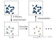
The initial position of the driving particle is the average of the positions of all its cluster members, where the number of driving particles is much smaller than the number of three-dimensional Gaussian particles.

During the rendering process, the position and rotation of each three-dimensional Gaussian particle are calculated by interpolating the position and rotation of the driving particle: for each three-dimensional Gaussian particle, first find its eight closest ones at time t=0 neighboring driven particles, and then fit the rigid body transformation T of these eight driven particles between time t=0 and the current timestamp to determine the current position and rotation of the particles.

Experimental results

Dataset

By capturing multiple perspectives Images, the researchers collected eight real-world static scenes, each of which included an object and a background. The items included five flowers (a red rose, a carnation, an orange rose, a tulip, and a (a white rose), an alocasia, a telephone cord, and a beanie; then capture four videos of the interactions to illustrate their natural movements after the interaction, such as poking or dragging, using real videos for additional comparison refer to.

Experimental results

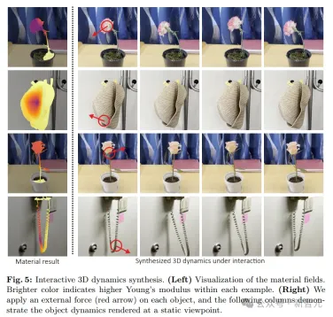
Regarding the spatially varying Young’s modulus ( A physical quantity that measures the elasticity of a material) Qualitative analysis results

In user studies, compared with baseline methods and real-world captured videos, it can be seen that there was more than 80% participation Participants preferred the PhysDreamer model in the two-choice experiment (2AFC), believing that it was superior in terms of realism of movement; in terms of visual quality, 65% of participants also preferred the PhysDreamer model

It should be noted that since the compared static scenes themselves are consistent, the evaluation of visual quality also relies on the motion effect of the generated objects to a certain extent.

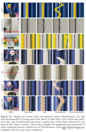
It can be observed from the slices of motion patterns at different time points that PhysGaussian is generated due to the lack of principled estimation of material properties. The range of motion is too large and the speed is too slow, which is inconsistent with reality.

Compared with DreamGaussian4D, 70% and 63.5% of the 2AFC samples prefer the PhysDreamer model in terms of visual quality and motion authenticity. As can be seen from the figure above, DreamGaussian4D The generated motion is periodic and the amplitude remains at a small constant value. In contrast, PhysDreamer can simulate the attenuation effect in motion.

The above is the detailed content of Hard core to solve Sora's physics bug! Four top universities in the United States jointly released: Install a physics engine for the video generator. For more information, please follow other related articles on the PHP Chinese website!