Summary of seven commonly used linear dimensionality reduction techniques in machine learning

In the previous article, we mainly summarized nonlinear dimensionality reduction techniques. In this article, we will summarize common linear dimensionality reduction techniques.

1. Principal Component Analysis (PCA)

PCA is a widely used dimensionality reduction technique that can convert high-dimensional data sets into more manageable low-dimensional representations while retaining the integrity of the data. Key Features. By identifying the directions (principal components) with the largest variance in the data, PCA can project the data into these directions to achieve the goal of dimensionality reduction.

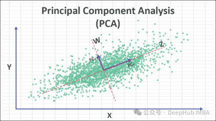
#The core idea of ​​PCA is to transform the original data into a new coordinate system to maximize the variance of the data. These new axes are called principal components and are linear combinations of the original features. Retaining the principal component with the largest variance essentially retains the key information of the data. By discarding the principal components with smaller variances, the purpose of dimensionality reduction can be achieved.

The steps of PCA are as follows:

1. Standardized data: Standardize the original data so that the mean of each feature is 0 and the variance is 1.
2. Calculate covariance matrix: Calculate the covariance matrix of the standardized data.
3. Calculate eigenvalues ​​and eigenvectors: Perform eigenvalue decomposition on the covariance matrix to obtain eigenvalues ​​and corresponding eigenvectors.
4. Select principal components: Select the first k eigenvectors as principal components according to the size of the eigenvalues, where k is the dimension after dimensionality reduction.
5. Projection data: Project the original data onto the selected principal components to obtain a dimensionally reduced data set.

PCA can be used for tasks such as data dimensionality reduction, feature extraction and pattern recognition. When using PCA, you need to ensure that the data meets the basic assumption of linear separability, and perform necessary data preprocessing and understanding to obtain accurate dimensionality reduction effects.

2. Factor Analysis (FA)

Factor Analysis (FA) is a statistical technique used to identify the underlying structure or factors among observed variables. It aims to uncover the latent factors that account for the shared variance among the observed variables, ultimately reducing them to a smaller number of unrelated variables.

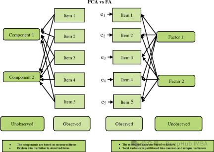
FA is somewhat similar to PCA, but there are also some important differences:

1. Objective: PCA aims to find the direction of maximum variance, while FA aims to find potential variables (factors) that can explain the common variation between the observed variables.
2. Assumptions: PCA assumes that the observed variables are the observed original features, while FA assumes that the observed variables are the linear combination of latent factors and the sum of random errors.
3. Interpretability: PCA tends to be more straightforward because its principal components are linear combinations of the original features. And the factors of FA may be less easy to interpret because they are linear combinations of observed variables rather than raw features.
4. Rotation: In FA, factors are often rotated to make them easier to interpret.

Factor analysis is widely used in fields such as psychology, social sciences, and market research. It helps simplify data sets, discover underlying structures, and reduce measurement errors. However, care needs to be taken in selecting the number of factors and rotation method to ensure that the results are interpretable and valid.

3. Linear Discriminant Analysis, LDA

Linear Discriminant Analysis (LDA) is a supervised learning technology used for dimensionality reduction and feature extraction. It is different from principal component analysis (PCA) because it not only considers the variance structure of the data, but also considers the category information of the data. LDA aims to find a projection direction that maximizes the distance between different categories (inter-class spread) while minimizing the distance within the same category (intra-class spread).

The main steps of LDA are as follows:

1. Calculate the mean vector of the category: For each category, calculate the mean vector of all samples under the category.
2. Calculate the within-class scatter matrix: For each category, calculate the scatter matrix between all samples under the category and its mean vector, and sum them.
3. Calculate the between-class scatter matrix: Calculate the scatter matrix between the mean vectors of all categories and the overall mean vector.
4. Calculate eigenvalues ​​and eigenvectors: Multiply the inverse matrix of the matrix by the inter-class scatter matrix, and perform eigenvalue decomposition of the resulting matrix to obtain eigenvalues ​​and eigenvectors.
5. Select the projection direction: Select the top k eigenvectors with the largest eigenvalues ​​as the projection direction, where k is the dimension after dimensionality reduction.
6. Projection data: Project the original data to the selected projection direction to obtain the dimensionally reduced data.

The advantage of LDA is that it takes into account the category information of the data, so the generated projection can better distinguish the differences between different categories. It is widely used in pattern recognition, face recognition, speech recognition and other fields. LDA may encounter some problems when dealing with multiple classes and class imbalance, and requires special attention.

4. Eigendecomposition

Eigendecomposition (eigenvalue decomposition) is a mathematical technique used to decompose square matrices. It decomposes a square matrix into a set of eigenvectors and the product of eigenvalues. Eigenvectors represent directions that do not change direction during transformations, while eigenvalues ​​represent scaling along these directions during transformations.

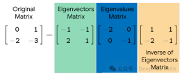
Given a square matrix AA, its eigenvalue decomposition is expressed as:

where Q is represented by A A matrix composed of eigenvectors, Λ is a diagonal matrix, and the elements on its diagonal are the eigenvalues ​​of A.

Eigenvalue decomposition has many applications, including principal component analysis (PCA), eigenface recognition, spectral clustering, etc. In PCA, eigenvalue decomposition is used to find the eigenvectors of the covariance matrix of the data and thus the principal components of the data. In spectral clustering, eigenvalue decomposition is used to find the eigenvectors of the similarity map, thereby performing clustering. Eigenface recognition uses eigenvalue decomposition to identify important features in face images.

Although eigenvalue decomposition is very useful in many applications, not all square matrices can be eigenvalue decomposed. For example, eigenvalue decomposition cannot be performed on singular matrices or non-square matrices. Eigenvalue decomposition can be very time-consuming to compute on large matrices.

5. Singular value decomposition (SVD)

Singular Value Decomposition (SVD) is an important technique for matrix decomposition. It decomposes a matrix into the product of three matrices, which are the transpose of an orthogonal matrix, a diagonal matrix, and another orthogonal matrix.

Given a m × n matrix AA, its singular value decomposition is expressed as:

where, U is an m × m orthogonal matrix , called the left singular vector matrix; Σ is an m × n diagonal matrix, and the elements on its diagonal are called singular values; VT is the transpose of an n × n orthogonal matrix, called the right singular vector matrix.

Singular value decomposition has a wide range of applications, including data compression, dimensionality reduction, matrix inverse solution, recommendation system, etc. In dimensionality reduction, only items with larger singular values ​​are retained, which can achieve effective compression and representation of data. In recommendation systems, the relationship between users and items can be modeled through singular value decomposition to provide personalized recommendations.

Singular value decomposition can also be used to solve matrix inverses, especially for singular matrices. By retaining the terms with larger singular values, the inverse matrix can be approximately solved, thereby avoiding the problem of inverting the singular matrix.

6. Truncated Singular Value Decomposition (TSVD)

Truncated Singular Value Decomposition (TSVD) is a variant of singular value decomposition (SVD), which is used in calculations Only the most important singular values ​​and corresponding singular vectors are retained to achieve dimensionality reduction and compression of data.

Given a m × n matrix AA, its truncated singular value decomposition is expressed as:

Where, Uk is an m × k orthogonal The matrix, Σk is a k × k diagonal matrix, VkT is the transpose of a k × n orthogonal matrix, these matrices correspond to preserving the most important k singular values ​​and the corresponding singular vectors.

The main advantage of TSVD is that it can achieve dimensionality reduction and compression of data by retaining the most important singular values ​​and singular vectors, thereby reducing storage and computing costs. This is particularly useful when working with large-scale data sets, as the required storage space and computation time can be significantly reduced.

TSVD has applications in many fields, including image processing, signal processing, recommendation systems, etc. In these applications, TSVD can be used to reduce the dimensionality of data, remove noise, extract key features, etc.

7. Non-Negative Matrix Factorization (NMF)

Non-Negative Matrix Factorization (NMF) is a technique for data decomposition and dimensionality reduction, which is characterized by the matrix obtained by decomposition and vectors are both non-negative. This makes NMF useful in many applications, especially in areas such as text mining, image processing, and recommender systems.

Given a non-negative matrix VV, NMF decomposes it into the product form of two non-negative matrices WW and HH:

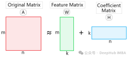
where, W is A non-negative matrix of m × k is called a basis matrix or feature matrix. H is a non-negative matrix of k × n, called a coefficient matrix. Here k is the dimension after dimensionality reduction.

The advantage of NMF is that it can obtain decomposition results with physical meaning because all elements are non-negative. This enables NMF to discover latent topics in text mining and extract features of images in image processing. In addition, NMF also has the function of data dimensionality reduction, which can reduce the dimensionality and storage space of data.

The applications of NMF include text topic modeling, image segmentation and compression, audio signal processing, recommendation systems, etc. In these fields, NMF is widely used in tasks such as data analysis and feature extraction, as well as information retrieval and classification.

Summary

Linear dimensionality reduction technology is a type of technology used to map high-dimensional data sets to low-dimensional space. Its core idea is to retain the main characteristics of the data set through linear transformation. These linear dimensionality reduction techniques have their unique advantages and applicability in different application scenarios, and the appropriate method can be selected based on the nature of the data and the requirements of the task. For example, PCA is suitable for unsupervised data dimensionality reduction, while LDA is suitable for supervised learning tasks.

Combined with the previous article, we introduced 10 nonlinear dimensionality reduction techniques and 7 linear dimensionality reduction techniques. Let’s make a summary

Linear dimensionality reduction technology: based on linear transformation Mapping data to a low-dimensional space is suitable for linearly separable data sets; for example, when data points are distributed on a linear subspace; because its algorithm is simple, the calculation is efficient and easy to understand and implement; it usually cannot capture the data The non-linear structure may lead to information loss.

Nonlinear dimensionality reduction technology: maps data to a low-dimensional space through nonlinear transformation; suitable for data sets with nonlinear structures, such as data points distributed on a manifold; can better retain data The nonlinear structure and local relationships in the image provide better visualization effects; the computational complexity is higher and usually requires more computing resources and time.

If the data is linearly separable or computing resources are limited, linear dimensionality reduction technology can be selected. If the data contains complex nonlinear structures or requires better visualization, you can consider using nonlinear dimensionality reduction technology. In practice, you can also try different methods and choose the most appropriate dimensionality reduction technology based on the actual effect.

The above is the detailed content of Summary of seven commonly used linear dimensionality reduction techniques in machine learning. For more information, please follow other related articles on the PHP Chinese website!