


Formula VLOOKUP is a very commonly used function in Microsoft Excel. It is used to find specific values in a table or data set and return other values associated with it. In this article, we will learn how to use the VLOOKUP formula correctly.
The basic syntax of the VLOOKUP function is as follows:
VLOOKUP(lookup_value, table_array, col_index_num, [range_lookup])
Among them:
- lookup_value: what you want to find Value, that is, the target value;
- table_array: The table or data set to be searched in needs to contain the column where the target value is located;
- col_index_num: The column where the target value is located is in the table or data Concentrated index number, counting from 1;
- range_lookup: optional parameter, used to specify the search method, TRUE indicates fuzzy matching (approximate matching), FALSE indicates exact matching. Defaults to TRUE.
Below we illustrate the use of the VLOOKUP formula through a practical example:
Suppose we have a sales order form that contains the product name, order quantity and unit price. We want to find the corresponding unit price based on the product name and calculate the total price.
First, we need to set up a separate area in the table to record all product names and corresponding unit prices. This area can be called the "Price List".
In the price list, we need to make sure that the columns where the product names are located are in alphabetical order. This ensures the normal operation of the VLOOKUP function.
Next, in the "Unit Price" column in the order form, we can apply the VLOOKUP function to find the unit price of the corresponding product. The specific operation is as follows:
- In the first cell of the "Unit Price" column, enter the starting part of the VLOOKUP function: =VLOOKUP(A2, price list,
- and then continue Enter the second parameter table_array, which is the cell range of the price list. We can directly select the entire price list, such as "$B$2:$C$10".
- Next, enter the third parameter col_index_num, That is, the index number of the column in the price list where the product unit price is located. In this example, we put the product unit price in the second column of the price list, so the index number is 2.
- Finally, we can Optionally enter the fourth parameter range_lookup to perform exact or fuzzy matching according to actual needs. In this example, we choose exact matching, so set this parameter to FALSE.
Complete the above steps, we will get something like The result in the picture below:
Product Name Order Quantity Unit Price
A 10 10
B 5 15
C 3 20
By using the VLOOKUP formula, in "Unit Price" We have successfully found the unit price of the corresponding product in the column. Next, we only need to multiply the "order quantity" and "unit price" to calculate the total price.
To summarize, the VLOOKUP formula is in Excel A very useful function that can help us quickly find target values in large data sets and return relevant data. Through the above examples, we can see the steps of using the VLOOKUP formula, which can help us improve work efficiency and reduce the number of manual searches. Time and errors. I hope this article will help everyone understand and use the VLOOKUP formula.
The above is the detailed content of How to use formula vlookup. For more information, please follow other related articles on the PHP Chinese website!

 计算机编程中常见的if语句是什么Jan 29, 2023 pm 04:31 PM
计算机编程中常见的if语句是条件判断语句。if语句是一种选择分支结构,它是依据明确的条件选择选择执行路径,而不是严格按照顺序执行,在编程实际运用中要根据程序流程选择适合的分支语句,它是依照条件的结果改变执行的程序;if语句的简单语法“if(条件表达式){// 要执行的代码;}”。
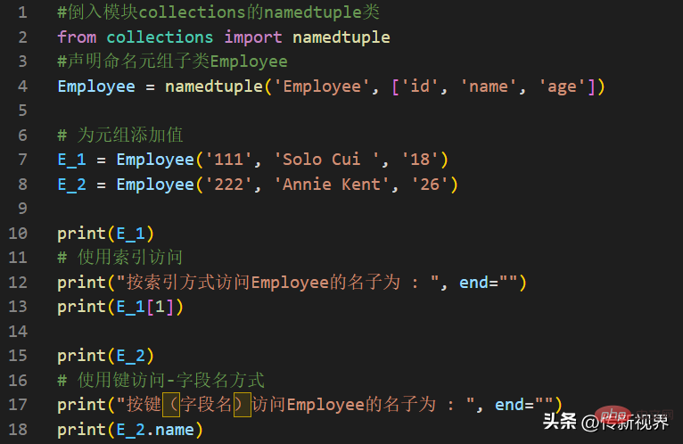 Python编程:详解命名元组(namedtuple)的使用要点Apr 11, 2023 pm 09:22 PM
前言本文继续来介绍Python集合模块,这次主要简明扼要的介绍其内的命名元组,即namedtuple的使用。闲话少叙,我们开始——记得点赞、关注和转发哦~ ^_^创建命名元组Python集合中的命名元组类namedTuples为元组中的每个位置赋予意义,并增强代码的可读性和描述性。它们可以在任何使用常规元组的地方使用,且增加了通过名称而不是位置索引方式访问字段的能力。其来自Python内置模块collections。其使用的常规语法方式为:import collections XxNamedT
 如何在Go中进行图像处理?May 11, 2023 pm 04:45 PM
作为一门高效的编程语言,Go在图像处理领域也有着不错的表现。虽然Go本身的标准库中没有提供专门的图像处理相关的API,但是有一些优秀的第三方库可以供我们使用,比如GoCV、ImageMagick和GraphicsMagick等。本文将重点介绍使用GoCV进行图像处理的方法。GoCV是一个高度依赖于OpenCV的Go语言绑定库,其
 PHP8.0中的邮件库May 14, 2023 am 08:49 AM
最近,PHP8.0发布了一个新的邮件库,使得在PHP中发送和接收电子邮件变得更加容易。这个库具有强大的功能,包括构建电子邮件,发送电子邮件,解析电子邮件,获取附件和解决电子邮件获得卡住的问题。在很多项目中,我们都需要使用电子邮件来进行通信和一些必备的业务操作。而PHP8.0中的邮件库可以让我们轻松地实现这一点。接下来,我们将探索这个新的邮件库,并了解如何在我
 PHP8.0中的DOMDocumentMay 14, 2023 am 08:18 AM
随着PHP8.0的发布,DOMDocument作为PHP内置的XML解析库,也有了新的变化和增强。DOMDocument在PHP中的重要性不言而喻,尤其在处理XML文档方面,它的功能十分强大,而且使用起来也十分简单。本文将介绍PHP8.0中DOMDocument的新特性和应用。一、DOMDocument概述DOM(DocumentObjectModel)
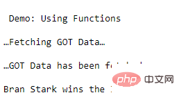 学Python,还不知道main函数吗Apr 12, 2023 pm 02:58 PM
Python 中的 main 函数充当程序的执行点,在 Python 编程中定义 main 函数是启动程序执行的必要条件,不过它仅在程序直接运行时才执行,而在作为模块导入时不会执行。要了解有关 Python main 函数的更多信息,我们将从如下几点逐步学习:什么是 Python 函数Python 中 main 函数的功能是什么一个基本的 Python main() 是怎样的Python 执行模式Let’s get started什么是 Python 函数相信很多小伙伴对函数都不陌生了,函数是可
 PHP8.0中的Symbol类型May 14, 2023 am 08:39 AM
PHP8.0是PHP语言的最新版本,自发布以来已经引发了广泛的关注和争议。其中,最引人瞩目的新特性之一就是Symbol类型。Symbol类型是PHP8.0中新增的一种数据类型,它类似于JavaScript中的Symbol类型,可用于表示独一无二的值。这意味着,两个Symbol类型的值即使完全相同,它们也是不相等的。Symbol类型的使用可以避免在不同的代码段
 PHP8.0中的HTTP客户端库May 14, 2023 am 08:51 AM
PHP8.0中的HTTP客户端库PHP8.0的发布带来了很多新特性和改进,其中一个最引人注目的是内置的HTTP客户端库的加入。这个库提供了一个简单的方法来发送HTTP请求并处理返回的响应。在本文中,我们将探讨这个库的主要功能和用法。发送HTTP请求使用PHP8.0内置的HTTP客户端库发送HTTP请求非常简单。在本例中,我们将使用GET方法获取这个网站的首页


Hot AI Tools

Undresser.AI Undress
AI-powered app for creating realistic nude photos

AI Clothes Remover
Online AI tool for removing clothes from photos.

Undress AI Tool
Undress images for free

Clothoff.io
AI clothes remover

AI Hentai Generator
Generate AI Hentai for free.

Hot Article
Hot Tools

WebStorm Mac version
Useful JavaScript development tools

DVWA
Damn Vulnerable Web App (DVWA) is a PHP/MySQL web application that is very vulnerable. Its main goals are to be an aid for security professionals to test their skills and tools in a legal environment, to help web developers better understand the process of securing web applications, and to help teachers/students teach/learn in a classroom environment Web application security. The goal of DVWA is to practice some of the most common web vulnerabilities through a simple and straightforward interface, with varying degrees of difficulty. Please note that this software

Zend Studio 13.0.1
Powerful PHP integrated development environment

Dreamweaver Mac version
Visual web development tools

Notepad++7.3.1
Easy-to-use and free code editor

