

Laplace approximation principle and its use cases in machine learning


The Laplace approximation is a numerical calculation method used to solve probability distributions in machine learning. It can approximate the analytical form of complex probability distributions. This article will introduce the principles, advantages and disadvantages of Laplace approximation, and its application in machine learning.
1. Laplace Approximation Principle
Laplace approximation is a method used to solve probability distribution, which uses The Taylor expansion approximates the probability distribution as a Gaussian distribution, thereby simplifying calculations. Suppose we have a probability density function $p(x)$ and we want to find its maximum value. We can approximate this using the following formula: $\hat{x} = \arg\max_x p(x) \approx \arg\max_x \log p(x) \approx \arg\max_x \left[\log p(x_0) (\nabla \log p(x_0 ))^T(x-x_0) - \frac{1}{2}(x-x_0)^T H(x-x_0)\right]$ Among them, $x_0$ is the maximum value point of $p(x)$, $\nabla \log p(x_0)$ is the gradient vector at $x_0$, and $H$ is the Hessian matrix at $x_0$. By solving the above equation
p(x)\approx\tilde{p}(x)=\frac{1}{(2\pi)^{D/2}|\ boldsymbol{H}|^{1/2}}\exp\left(-\frac{1}{2}(\boldsymbol{x}-\boldsymbol{\mu})^T\boldsymbol{H}(\boldsymbol {x}-\boldsymbol{\mu})\right)
In this approximation, $\boldsymbol{\mu}$ represents the probability density function $p(x)$ The maximum value point of $\boldsymbol{H}$ represents the Hessian matrix of $p(x)$ at $\boldsymbol{\mu}$, and $D$ represents the dimension of $x$. This approximation can be viewed as a Gaussian distribution, where $\boldsymbol{\mu}$ is the mean and $\boldsymbol{H}^{-1}$ is the covariance matrix.
It is worth noting that the accuracy of the Laplace approximation depends on the shape of p(x) at \boldsymbol{\mu}. This approximation is very accurate if p(x) is close to a Gaussian distribution at \boldsymbol{\mu}. Otherwise, the accuracy of this approximation will be reduced.
2. Advantages and disadvantages of Laplace approximation
The advantages of Laplace approximation are:
- For the case of Gaussian distribution approximation, the accuracy is very high.
- The calculation speed is faster, especially for high-dimensional data.
- can be used to analyze the maximum value of the probability density function, and to calculate statistics such as expectation and variance.
The disadvantage of Laplace approximation is:
- ##For non-Gaussian distribution, the approximation accuracy will be reduced .
- The approximation formula can only be applied to a local maximum point, but cannot handle the situation of multiple local maximum values.
- The solution to the Hessian matrix \boldsymbol{H} requires calculation of the second-order derivative, which requires the existence of the second-order derivative of p(x) at \boldsymbol{\mu}. Therefore, if higher-order derivatives of p(x) do not exist or are difficult to compute, the Laplace approximation cannot be used.
The above is the detailed content of Laplace approximation principle and its use cases in machine learning. For more information, please follow other related articles on the PHP Chinese website!

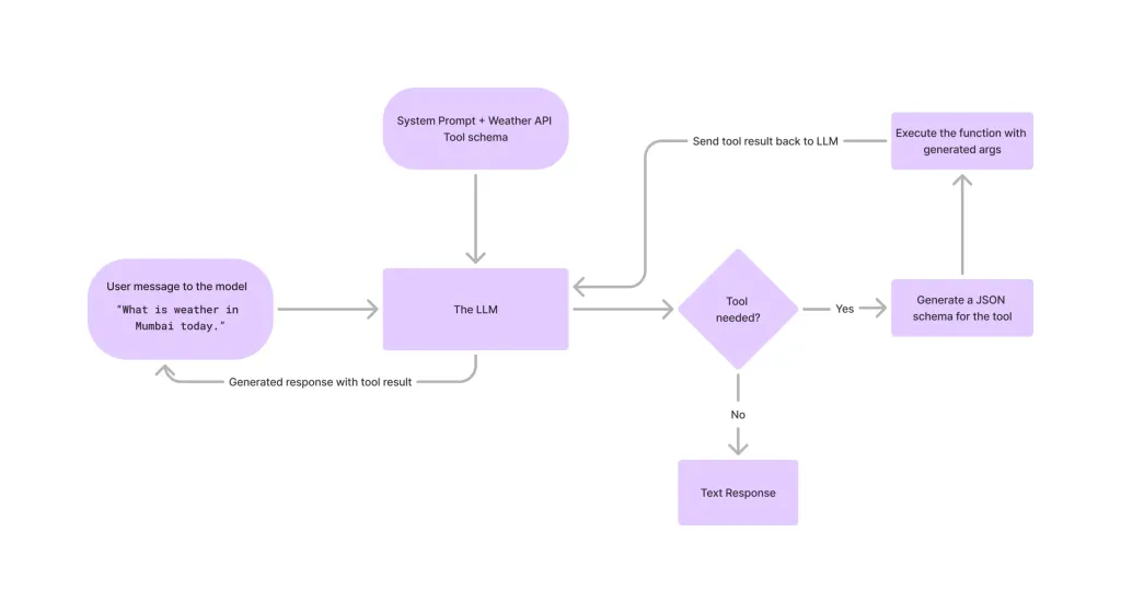 Tool Calling in LLMsApr 14, 2025 am 11:28 AM
Large language models (LLMs) have surged in popularity, with the tool-calling feature dramatically expanding their capabilities beyond simple text generation. Now, LLMs can handle complex automation tasks such as dynamic UI creation and autonomous a
 How ADHD Games, Health Tools & AI Chatbots Are Transforming Global HealthApr 14, 2025 am 11:27 AM
Can a video game ease anxiety, build focus, or support a child with ADHD? As healthcare challenges surge globally — especially among youth — innovators are turning to an unlikely tool: video games. Now one of the world’s largest entertainment indus
 UN Input On AI: Winners, Losers, And OpportunitiesApr 14, 2025 am 11:25 AM
“History has shown that while technological progress drives economic growth, it does not on its own ensure equitable income distribution or promote inclusive human development,” writes Rebeca Grynspan, Secretary-General of UNCTAD, in the preamble.
 Learning Negotiation Skills Via Generative AIApr 14, 2025 am 11:23 AM
Easy-peasy, use generative AI as your negotiation tutor and sparring partner. Let’s talk about it. This analysis of an innovative AI breakthrough is part of my ongoing Forbes column coverage on the latest in AI, including identifying and explaining
 TED Reveals From OpenAI, Google, Meta Heads To Court, Selfie With MyselfApr 14, 2025 am 11:22 AM
The TED2025 Conference, held in Vancouver, wrapped its 36th edition yesterday, April 11. It featured 80 speakers from more than 60 countries, including Sam Altman, Eric Schmidt, and Palmer Luckey. TED’s theme, “humanity reimagined,” was tailor made
 Joseph Stiglitz Warns Of The Looming Inequality Amid AI Monopoly PowerApr 14, 2025 am 11:21 AM
Joseph Stiglitz is renowned economist and recipient of the Nobel Prize in Economics in 2001. Stiglitz posits that AI can worsen existing inequalities and consolidated power in the hands of a few dominant corporations, ultimately undermining economic
 What is Graph Database?Apr 14, 2025 am 11:19 AM
Graph Databases: Revolutionizing Data Management Through Relationships As data expands and its characteristics evolve across various fields, graph databases are emerging as transformative solutions for managing interconnected data. Unlike traditional
 LLM Routing: Strategies, Techniques, and Python ImplementationApr 14, 2025 am 11:14 AM
Large Language Model (LLM) Routing: Optimizing Performance Through Intelligent Task Distribution The rapidly evolving landscape of LLMs presents a diverse range of models, each with unique strengths and weaknesses. Some excel at creative content gen


Hot AI Tools

Undresser.AI Undress
AI-powered app for creating realistic nude photos

AI Clothes Remover
Online AI tool for removing clothes from photos.

Undress AI Tool
Undress images for free

Clothoff.io
AI clothes remover

AI Hentai Generator
Generate AI Hentai for free.

Hot Article
Hot Tools

Atom editor mac version download
The most popular open source editor

ZendStudio 13.5.1 Mac
Powerful PHP integrated development environment

Safe Exam Browser
Safe Exam Browser is a secure browser environment for taking online exams securely. This software turns any computer into a secure workstation. It controls access to any utility and prevents students from using unauthorized resources.

EditPlus Chinese cracked version
Small size, syntax highlighting, does not support code prompt function

Dreamweaver CS6
Visual web development tools

