Break through the information barrier! Shocking large-scale 3D visualization tool is released!

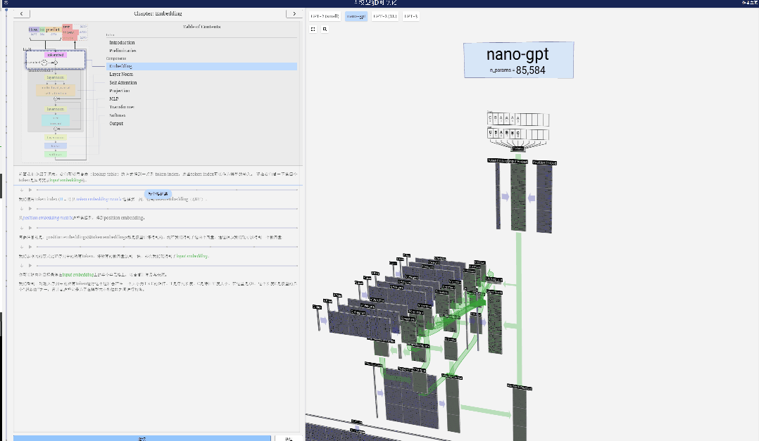
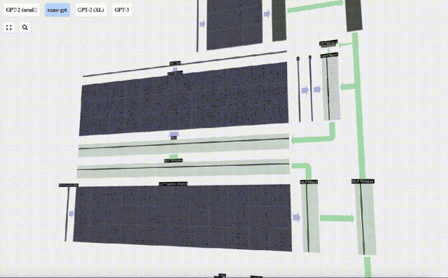
Recently, a young man from New Zealand, Brendan Bycroft, has set off a craze in the technology circle. A project he created called Large Model 3D Visualization not only topped the list of Hacker News, but its shocking effect is even more jaw-dropping. Through this project, you will fully understand how LLM (Large Language Model) works in just a few seconds.

Whether you are a technology enthusiast or not, this project will bring you an unprecedented visual feast and cognitive enlightenment. Let’s explore this stunning creation together!

Introduction

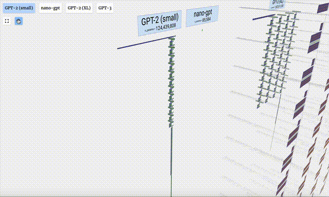
In this project, Bycroft analyzed in detail a lightweight GPT model called Nano-GPT developed by OpenAI scientist Andrej Karpathy. As a reduced version of the GPT model, the model only has 85,000 parameters. Of course, although this model is much smaller than OpenAI's GPT-3 or GPT-4, it can be said that "a sparrow is small but has all the internal organs."

Nano-GPT GitHub: https://github.com/karpathy/nanoGPT

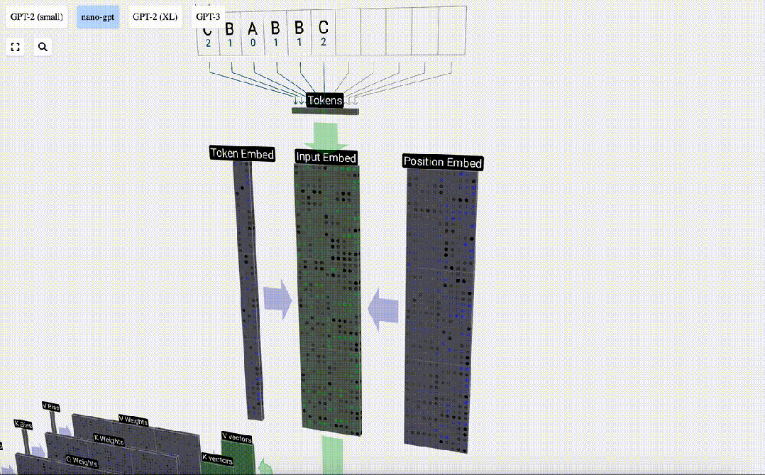
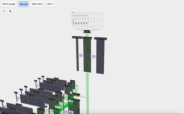
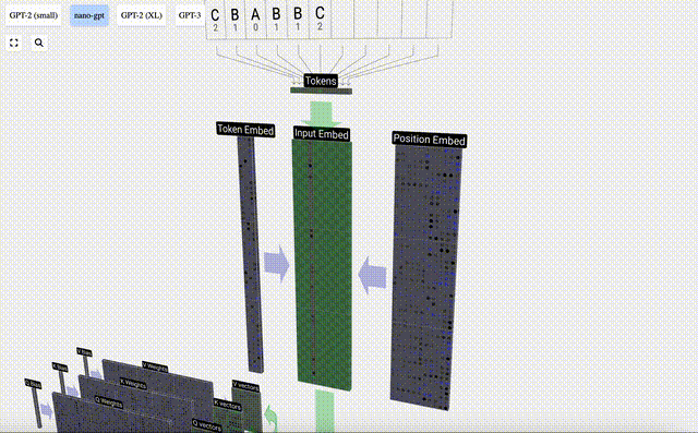
In order to facilitate the demonstration of each layer of the Transformer model, Bycroft arranged a very simple target for the Nano-GPT model Task: The model input is the 6 letters "CBABBC", and the output is a sequence arranged in alphabetical order, for example, the output is "ABBBCC".

We call each letter a token , these different letters constitute the vocabulary vocabulary:

For this table, each letter is assigned a subscript token index. The sequence composed of these subscripts can be used as the input of the model: 2 1 0 1 1 2

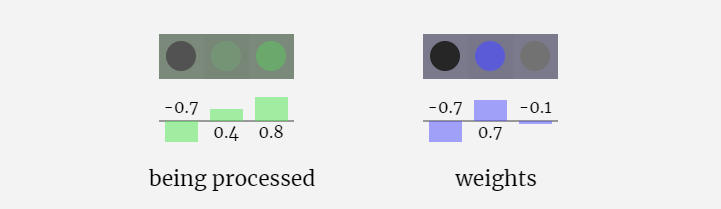
In the 3D visualization, each green cell represents a calculated number, and each The blue cells represent the weights of the model.

#In sequence processing, each number is first converted into a C-dimensional vector. This process is called embedding. In Nano-GPT, the dimension of this embedding is usually 48 dimensions. Through this embedding operation, each number is represented as a vector in C-dimensional space, which enables better subsequent processing and analysis.

embedding goes through a series of intermediate model layer calculations, which are generally called Transformers, and finally reaches the bottom layer.

"So what is the output?"

The output of the model is the next token in the sequence. So at the end, we get the probability value that the next token is A B C.

In this example, the 6th position model outputs A with a high probability. Now we can pass A as input to the model and repeat the whole process.

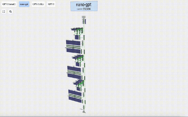
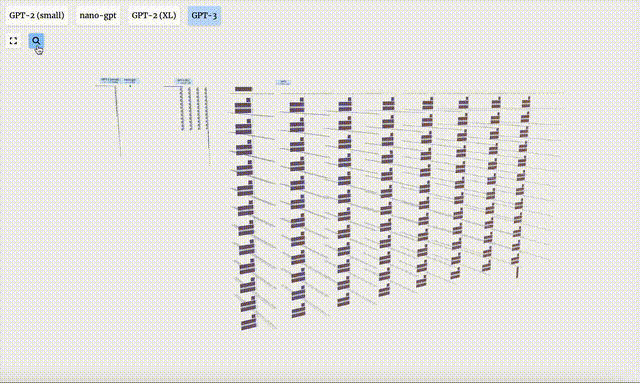
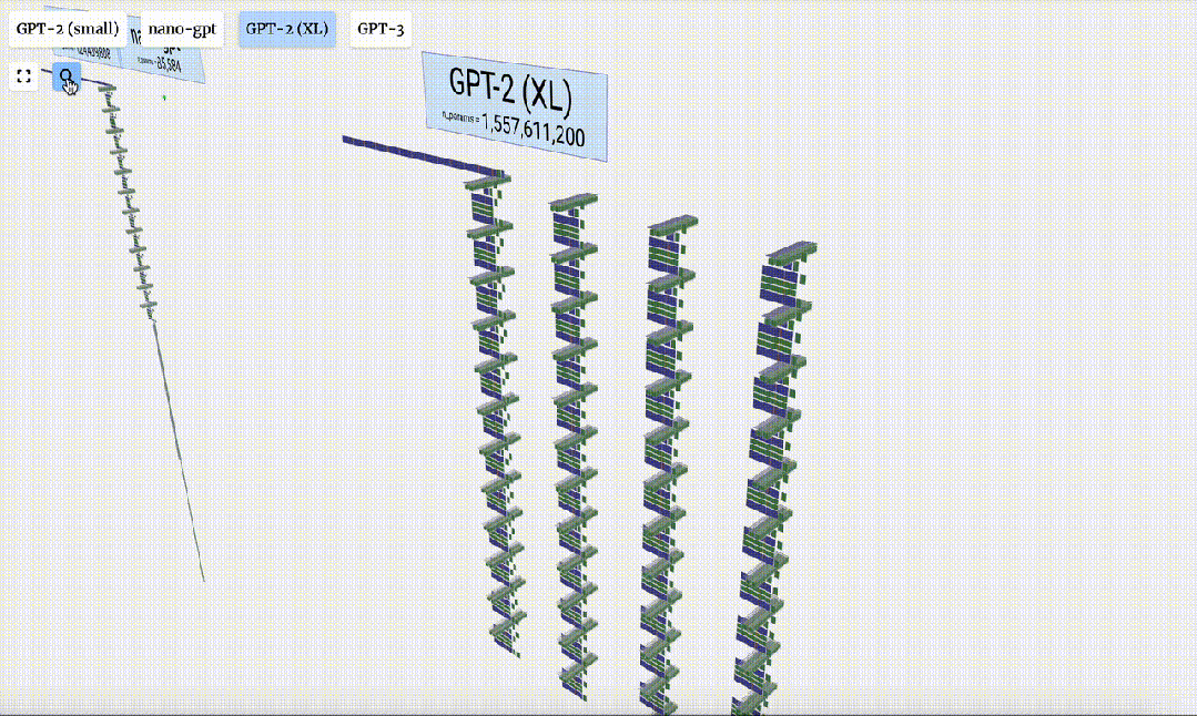
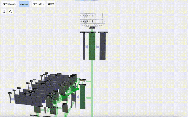
In addition, GPT-2 and GPT-3 visualization effects are also displayed.

• GPT-3 has 175 billion parameters, and the model layer has 8 columns, densely covering the entire screen.

• Different parameter versions of the GPT-2 model show huge architectural differences. Here we take the 15 billion parameters of GPT-2 (XL) and the 124 million parameters of GPT-2 (Small) as examples.

It should be noted that this visualization mainly focuses on model inference (inference) rather than training, so it Just a small part of the overall machine learning process. Moreover, it is assumed here that the weights of the model have been pre-trained, and then model inference is used to generate output.

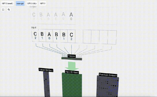
Embedding

As mentioned earlier, how to use a simple lookup table (Lookup Table) to map tokens to a series of integers.

These integers, the token index, are the first and only time the model sees integers. After that, operations will be performed using floating point numbers (decimal numbers).

Here, take the 4th token (index 3) as an example to see how it is used to generate the 4th column vector of the input embedding.

First use the token index (here, B=1 is used as an example) to select the second column from the Token Embedding matrix and get a column of size C=48 (48 dimensions) Vector, called token embedding.

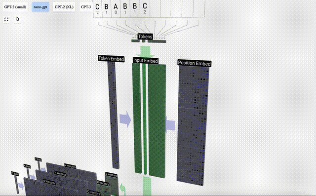
Then select the fourth column from the position embedding matrix ("Because here we mainly look at the (t = 3) token B at the 4th position"), similarly, we get a A column vector of size C=48 (48 dimensions) is called position embedding.

It should be noted that position embeddings and token embeddings are both obtained by model training (indicated by blue). Now that we have these two vectors, by adding them we can get a new column vector of size C=48.

Next, process all tokens in the sequence in the same process, creating a set of vectors containing the token values ​​and their positions.

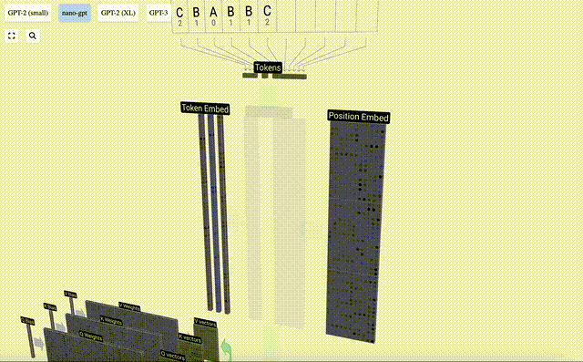
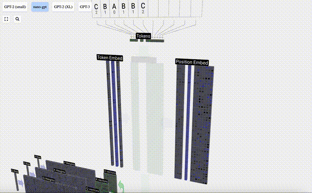
As can be seen from the above figure, running this process on all tokens in the input sequence will produce a matrix of size TxC. Among them, T represents the sequence length. C stands for channel, but is also called feature or dimension or embedding size, which in this case is 48. This length C is one of several "hyperparameters" of the model, chosen by the designer to provide a trade-off between model size and performance.

This matrix with dimension TxC is the input embedding and is passed down through the model.

Little Tip: Feel free to hover your mouse over a single cell on the input embedding to see the calculation and its source.

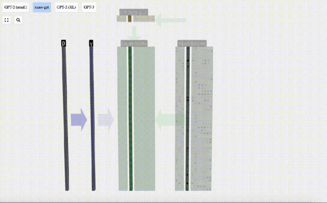
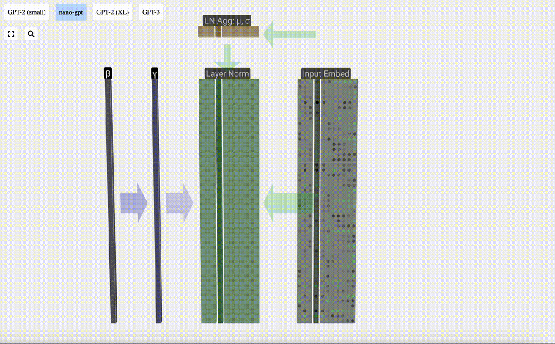
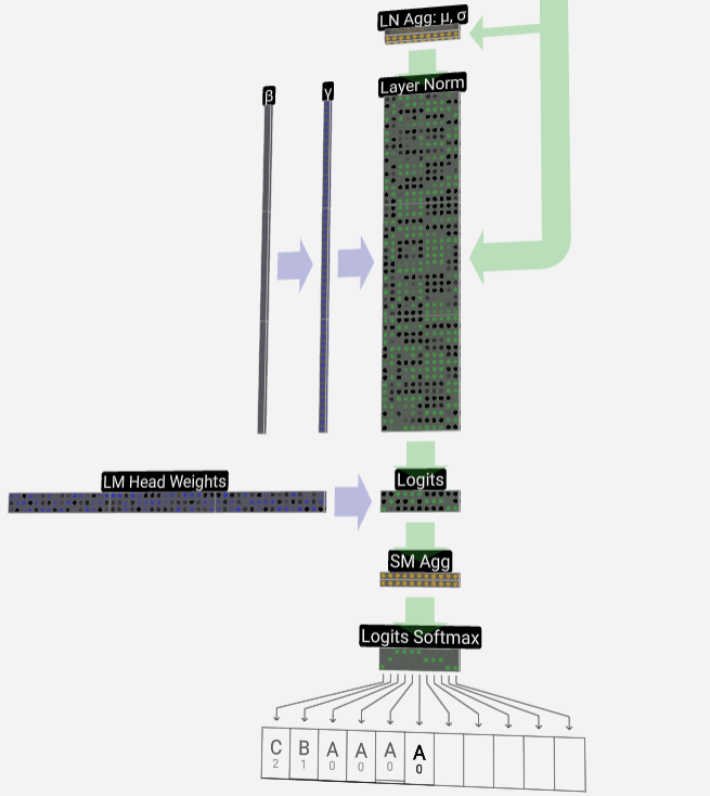
Layer Normalization Layer Norm

The input embedding matrix obtained previously is the input of the Transformer layer.

The first step of the Transformer layer is to perform layer normalization on the input embedding matrix. This is an operation to normalize the values ​​of each column of the input matrix.

Normalization is an important step in deep neural network training, which helps improve the stability of the model during the training process.

We can look at the columns of the matrix separately. The fourth column is taken as an example below.

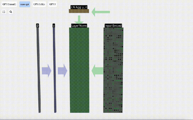
The goal of normalization is to make the mean value of each column is 0 and the standard deviation is 1. To achieve this, calculate the mean and standard deviation of each column, and then subtract the corresponding mean and divide by the corresponding standard deviation for each column.

E[x] is used here to represent the mean, and Var[x] is used to represent the variance (the square of the standard deviation). epsilon(ε = 1×10^-5) is to prevent division by 0 errors.

Calculate and store the normalized result, then multiply it by the learning weight weight(γ) and add the bias bias(β) to obtain the final normalized result.

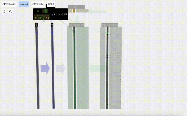
Finally, perform the normalization operation on each column of the input embedding matrix to obtain the normalized input embedding. ) and pass it to the self-attention layer.

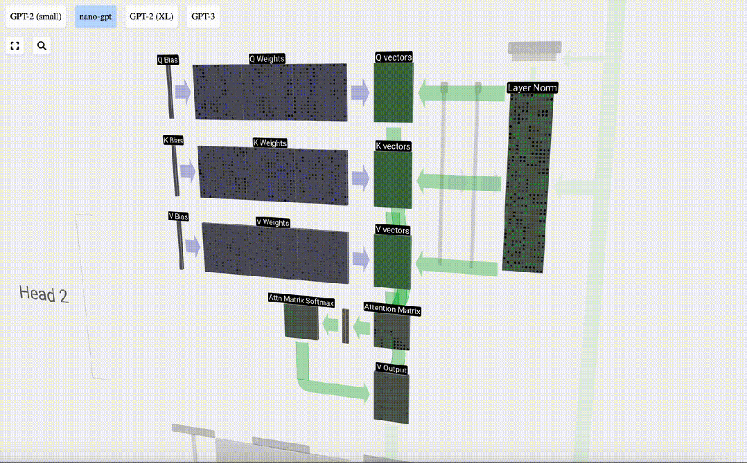
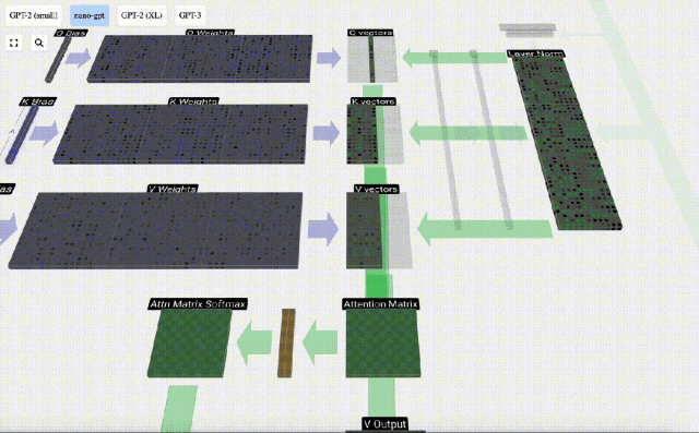
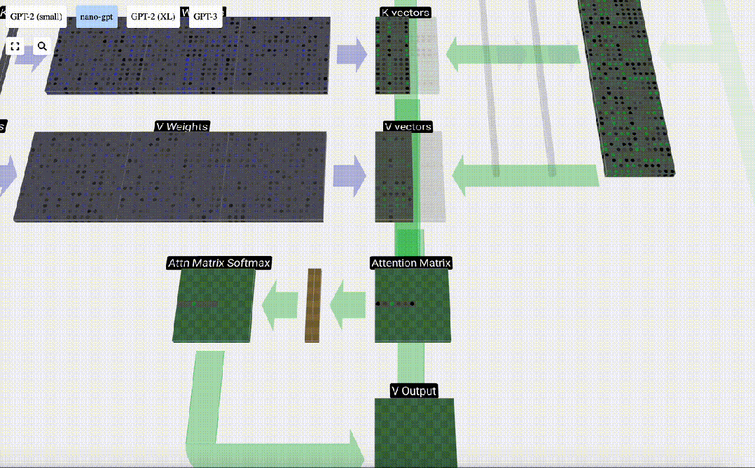
Self Attention

The Self Attention layer is probably the core part of the Transformer. At this stage, the columns in the input embedding can "communicate" with each other, while in other stages, each column is exists independently.

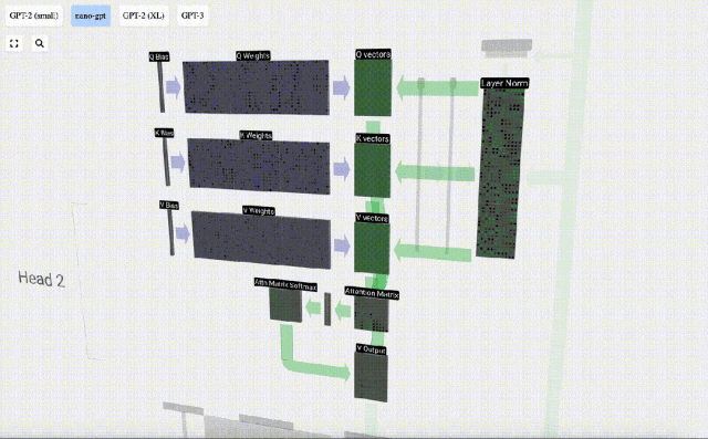
The Self Attention layer is composed of multiple self-attention heads. In this example, there are three self-attention heads. The input of each header is 1/3 of the input embedding, and we only focus on one of them now.

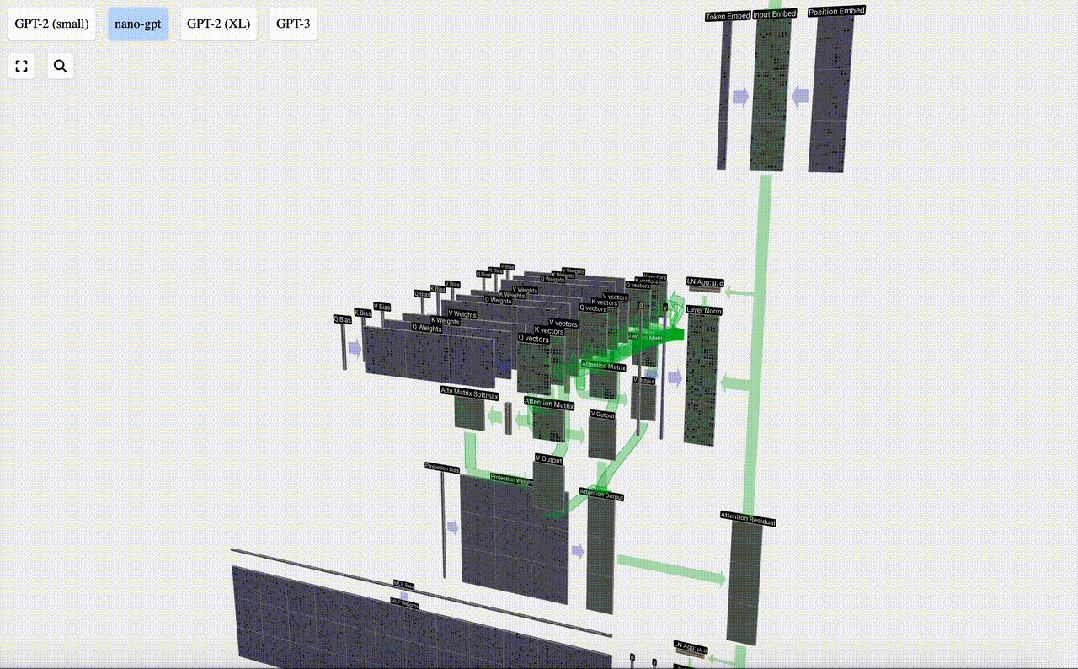
The first step is to generate 3 vectors for each column from column C of the normalized input embedding matrix, which are QKV:

• Q : Query vector
• K: Key vector Key vector
• V: Value vector Value vector

To generate these vectors, matrix-vector multiplication is required, Added bias. Each output unit is a linear combination of input vectors.

For example, for the query vector, it is completed by the dot product operation between a row of the Q weight matrix and a column of the input matrix.

#The operation of dot product is very simple, that is, multiply the corresponding elements and then add them.

This is a general and simple way to ensure that each output element is affected by all elements in the input vector (this influence is determined by the weight). Therefore, it often appears in neural networks.

In neural networks, this mechanism often occurs because it allows the model to take into account every part of the input sequence when processing the data. This comprehensive attention mechanism is at the core of many modern neural network architectures, especially when processing sequential data such as text or time series.

We repeat this for each output unit in the Q, K, V vectors:

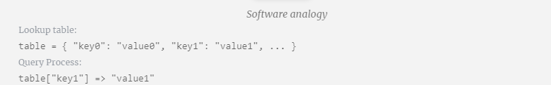
How we use our Q (query), K What about the (key) and V (value) vectors? Their naming gives us a hint: 'key' and 'value' are reminiscent of dictionary types, with keys mapping to values. Then 'query' is what we use to find the value.

In the case of Self Attention, instead of returning a single vector (term), we return some weighted combination of vectors (terms). To find this weight, we calculate the dot product between a Q vector and each K vector, weight and normalize it, and finally multiply it by the corresponding V vector and add them together.

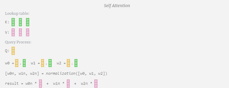
Taking the 6th column as an example (t=5), the query will start from this column:

Because Due to the existence of attention matrix, the first 6 columns of KV can be queried, and the Q value is the current time.

First calculate the dot product between the Q vector of the current column (t=5) and the K vector of the previous columns (the first 6 columns). This is then stored in the corresponding row (t=5) of the attention matrix.

#The size of the dot product measures the similarity between two vectors. The larger the dot product, the more similar they are.

And only the Q vector is operated with the past K vector, making it a causal self-attention. In other words, tokens cannot ‘see future information’.

Therefore, after finding the dot product, divide by sqrt(A), where A is the length of the QKV vector. This scaling is done to prevent large values ​​from being used in the next step of normalization (softmax) Dominant.

Next, the softmax operation is performed to reduce the value range to 0 to 1.

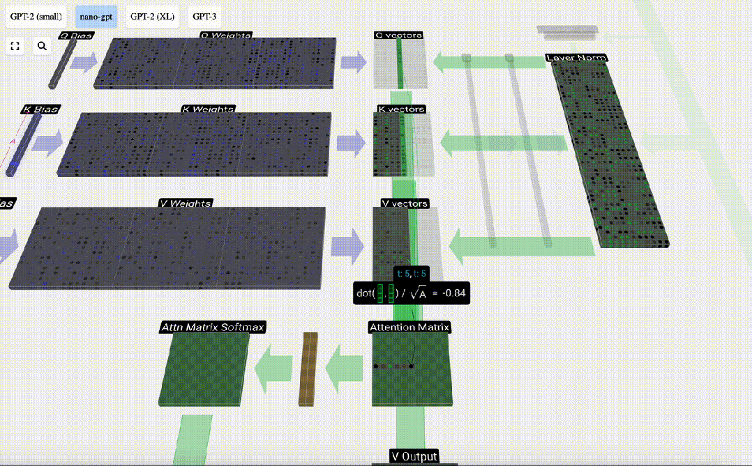
#Finally, you can get the output vector of this column (t=5). Look at the (t=5) row of the normalized attention matrix and multiply each element with the corresponding V vector of the other column.

We can then add these vectors to get the output vector. Therefore, the output vector will be dominated by the V vector with high resolution.

Now we apply it to all columns.

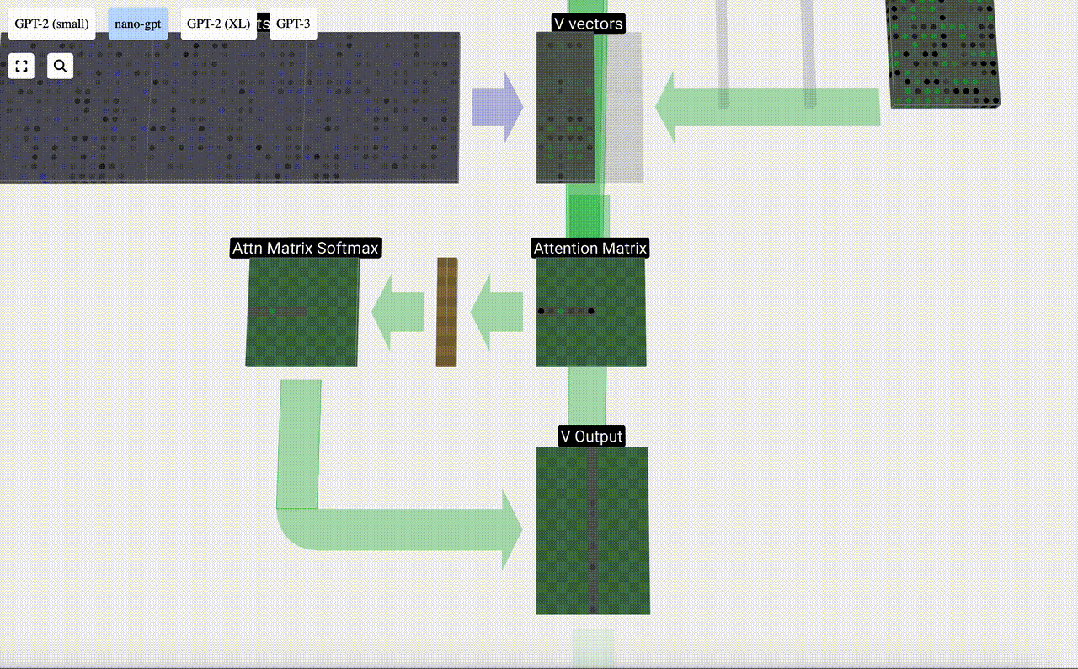
This is the processing process of a header in the Self Attention layer. "So the main goal of Self Attention is that each column wants to find relevant information from other columns and extract its value, and it does this by comparing its Query vector with the Keys of those other columns. The added limitation is that it only Can look into the past."

Projection

After the Self Attention operation, we will get an output from each head. These outputs are V vectors that are appropriately blended, influenced by the Q and K vectors. To merge the output vectors of each head, we simply stack them together. Therefore, at t=4, we will superpose 3 vectors with length A=16 to form 1 vector with length C=48.

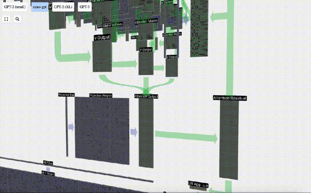
It is worth noting that in GPT, the length of the vector within the head (A=16) is equal to C/num_heads. This ensures that when we stack them back together, we get the original length C.

Based on this, we perform projection and get the output of this layer. This is a simple matrix-vector multiplication, per column, plus a bias.

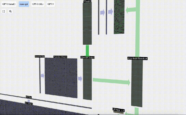
Now we have the output of Self Attention.

We do not pass this output directly to the next stage, but add it to the input embedding as an element. This process, represented by the green vertical arrow, is called the residual connection or residual pathway.

Like Layer Normalization, residual networks are crucial to achieve effective learning of deep neural networks.

Now that we have the result of self-attention, we can pass it to the next layer of Transformer: the feedforward network.

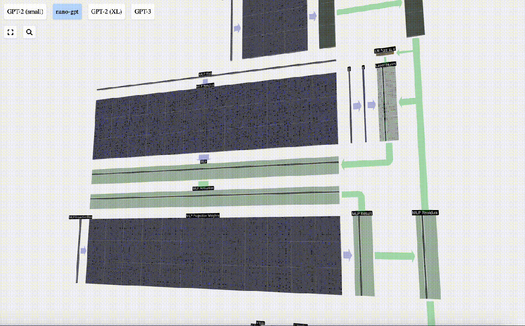
Multilayer Perceptron MLP

After Self Attention, the next part of the Transformer module is MLP (Multilayer Perceptron), here it is a simple neural network with two layers.

Like Self Attention, we need to perform layer normalization before the vector enters the MLP.

At the same time, in MLP, each column vector with length C=48 needs to be processed (independently) as follows:

• Add a linear transformation with bias ( That is, matrix-vector multiplication plus an offset operation), converted into a vector of length 4 * C.
• GELU activation function (applied element-wise).
• Perform linear transformation with bias, and then transform it back into a vector of length C.

Let us trace one of the vectors:

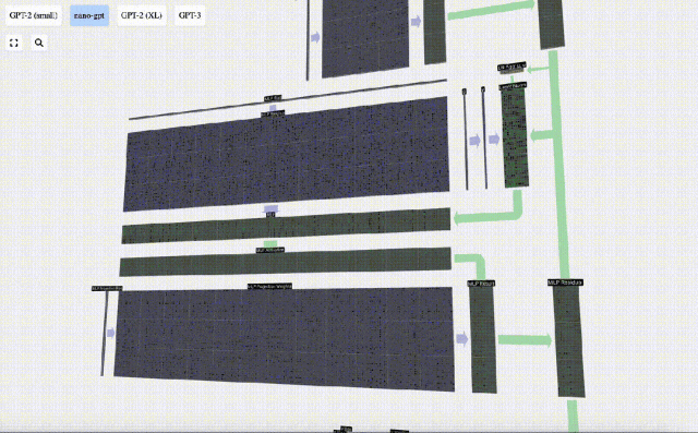
The MLP process is as follows:

First perform matrix-vector multiplication and Adding biases expands the vector into a matrix of length 4*C. (Note that the output matrix here is transposed for visualization)

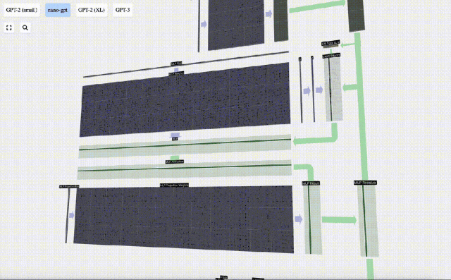
Next, apply the GELU activation function to each element of the vector. This is a key part of any neural network, we need to introduce some non-linearity into the model. The specific function used, GELU, looks a lot like the ReLU function max(0, x), but it has a smooth curve instead of sharp corners.

The vector is then projected back to length C via another biased matrix-vector multiplication.

There is also a residual network here. Like the self-attention projection part, we add the results of the MLP to the input in element order.

Repeat these operations.

#The MLP layer ends here, and we finally get the output of the transformer.

Transformer

This is a complete Transformer module!

These several modules constitute the main body of any GPT model, and the output of each module is the output of the next module. enter.

As is common in deep learning, it’s hard to tell exactly what each of these layers is doing, but we have some general ideas: earlier layers tend to focus on learning low-level features and patterns, while later layers tend to focus on learning low-level features and patterns. The layers learn to recognize and understand higher-level abstractions and relationships. In the context of natural language processing, lower layers may learn grammar, syntax, and simple lexical associations, while higher layers may capture more complex semantic relationships, discourse structures, and context-dependent meanings.

Softmax

The last step is the softmax operation, which outputs the predicted probability of each token.

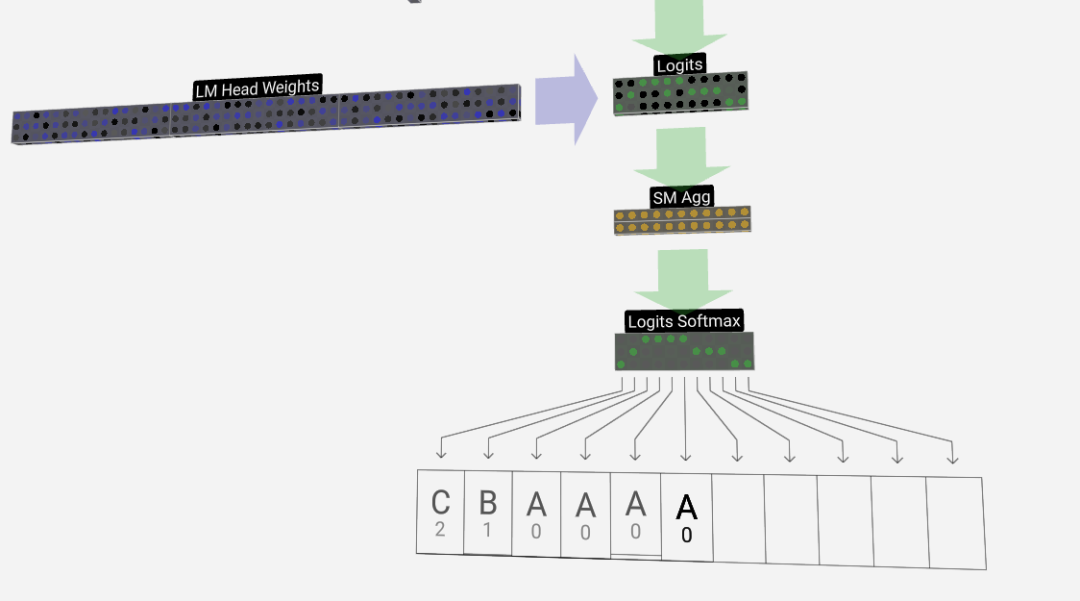
Output

Finally, we reach the end of the model. The output of the last Transformer undergoes a layer of regularization, followed by an unbiased linear transformation.

This final transformation transforms each of our column vectors from length C to vocabulary-sized length nvocab. So it actually generates a score logits for each word in the vocabulary.

In order to convert these scores into more intuitive probability values, they need to be processed through softmax first. So, for each column, we get the probability that the model assigned to each word in the vocabulary.

In this particular model, it has actually learned all the answers on how to order the three letters, so the probabilities are heavily tilted towards the correct answer.

When we let the model advance over time, we need to use the probability of the last column to determine the next added token in the sequence. For example, if we input six tokens into the model, we would use the output probabilities in column six.

The output of this column is a series of probability values, from which we actually need to select one as the next token in the sequence. We achieve this by "sampling from the distribution", that is, randomly selecting a token based on its probability. For example, a token with probability 0.9 has a 90% probability of being selected. However, we also have other options, such as always choosing the token with the highest probability.

We can also control the "smoothness" of the distribution by using the temperature parameter. Higher temperatures will make the distribution more even, while lower temperatures will make it more concentrated on the tokens with the highest probability.

We adjust logits (the output of the linear transformation) by using the temperature parameter before applying softmax, because the exponentiation in softmax has a significant amplification effect on larger values, making all values ​​closer will reduce this kind of effect.

picture

The above is the detailed content of Break through the information barrier! Shocking large-scale 3D visualization tool is released!. For more information, please follow other related articles on the PHP Chinese website!