
Home >Technology peripherals >AI >Link prediction code example using Pytorch Geometric
Link prediction code example using Pytorch Geometric

- 王林forward
- 2023-10-20 19:33:081330browse
PyTorch Geometric (PyG) is the main tool for building graph neural network models and experimenting with various graph convolutions. In this article we will introduce it through link prediction.

Link prediction answers the question: Which two nodes should be linked to each other? We will prepare the data for modeling by performing a "transformation split". Prepare dedicated graph data loader for batch processing. Build a model in Torch Geometric, train it using PyTorch Lightning, and check the model's performance.
Library preparation
- Torch No need to introduce more
- Torch Geometric graphical neural network's main library is also the focus of this article
- PyTorch Lightning is used to train, tune, and validate models. It simplifies the operation of training
- Sklearn Metrics and Torchmetrics are used to check the performance of the model.
- PyTorch Geometric has some specific dependencies, if you have problems installing it, please refer to its official documentation.
Data preparation
We will use the Cora ML citation dataset. The dataset can be accessed through Torch Geometric.
data = tg.datasets.CitationFull(root="data", name="Cora_ML")
By default, the Torch Geometric dataset can return multiple graphs. Let's see what a single graph looks like
data[0] > Data(x=[2995, 2879], edge_index=[2, 16316], y=[2995])
Here X is the characteristic of the node. edge_index is a 2 x (n edges) matrix (first dimension = 2, interpreted as: row 0 - source node/"sender", row 1 - target node/"receiver").
Link Splitting
We will start by splitting the links in the dataset. Use 20% of the graph links as the validation set and 10% as the test set. Negative samples will not be added to the training dataset here as such negative links will be created on the fly by the batch data loader.
Generally speaking, negative sampling creates "fake" samples (in our case links between nodes), so the model learns how to distinguish between real and fake links. Negative sampling is based on the theory and mathematics of sampling and has some nice statistical properties.
First: let’s create a link split object.
link_splitter = tg.transforms.RandomLinkSplit(num_val=0.2, num_test=0.1, add_negative_train_samples=False,disjoint_train_ratio=0.8)
disjoint_train_ratio adjusts how many edges will be used as training information in the "supervision" phase. The remaining edges will be used for message passing (the information transfer phase in the network).
There are at least two methods of segmenting edges in graph neural networks: inductive segmentation and conductive segmentation. The transformation method assumes that GNN needs to learn structural patterns from graph structures. In an inductive setting, node/edge labels can be used for learning. There are two papers at the end of this paper that discuss these concepts in detail and provide additional formalization: ([1], [3]).
train_g, val_g, test_g = link_splitter(data[0]) > Data(x=[2995, 2879], edge_index=[2, 2285], y=[2995], edge_label=[9137], edge_label_index=[2, 9137])
After this operation, we have some new attributes:
edge_label: describes whether the edge is true/false. This is what we want to predict.
edge_label_index is a 2 x NUM EDGES matrix used to store node links.
Let's look at the distribution of samples
th.unique(train_g.edge_label, return_counts=True) > (tensor([1.]), tensor([9137])) th.unique(val_g.edge_label, return_counts=True) > (tensor([0., 1.]), tensor([3263, 3263])) th.unique(val_g.edge_label, return_counts=True) > (tensor([0., 1.]), tensor([3263, 3263]))
For the training data there are no negative edges (we will create them while training), for the val/test set - already in the ratio of 50:50 There are some "fake" links.
Model
Now we can use GNN to build a model and build a
class GNN(nn.Module):
def __init__(self, dim_in: int, conv_sizes: Tuple[int, ...], act_f: nn.Module = th.relu, dropout: float = 0.1,*args, **kwargs):super().__init__()self.dim_in = dim_inself.dim_out = conv_sizes[-1]self.dropout = dropoutself.act_f = act_flast_in = dim_inlayers = [] # Here we build subsequent graph convolutions.for conv_sz in conv_sizes:# Single graph convolution layerconv = tgnn.SAGEConv(in_channels=last_in, out_channels=conv_sz, *args, **kwargs)last_in = conv_szlayers.append(conv)self.layers = nn.ModuleList(layers) def forward(self, x: th.Tensor, edge_index: th.Tensor) -> th.Tensor:h = x# For every graph convolution in the network...for conv in self.layers:# ... perform node embedding via message passingh = conv(h, edge_index)h = self.act_f(h)if self.dropout:h = nn.functional.dropout(h, p=self.dropout, training=self.training)return h
This model is worth The part of interest is a set of graph convolutions - in our case SAGEConv. The formal definition of SAGE convolution is:
 å¾ç
å¾ç
v is the current node and the N(v) neighbors of node v. To learn more about this type of convolution, check out the original paper from GraphSAGE[1]
Let’s check if the model can make predictions using prepared data. The input to the PyG model here is the matrix of node features X and the link defining edge_index.
gnn = GNN(train_g.x.size()[1], conv_sizes=[512, 256, 128]) with th.no_grad():out = gnn(train_g.x, train_g.edge_index) out > tensor([[0.0000, 0.0000, 0.0051, ..., 0.0997, 0.0000, 0.0000],[0.0107, 0.0000, 0.0576, ..., 0.0651, 0.0000, 0.0000],[0.0000, 0.0000, 0.0102, ..., 0.0973, 0.0000, 0.0000],...,[0.0000, 0.0000, 0.0549, ..., 0.0671, 0.0000, 0.0000],[0.0000, 0.0000, 0.0166, ..., 0.0000, 0.0000, 0.0000],[0.0000, 0.0000, 0.0034, ..., 0.1111, 0.0000, 0.0000]])
The output of our model is a node embedding matrix with dimensions: N nodes x embedding size.
PyTorch Lightning
PyTorch Lightning is mainly used for training, but here we add a Linear layer after the output of the GNN as the output head for predicting whether to link.
class LinkPredModel(pl.LightningModule):
def __init__(self,dim_in: int,conv_sizes: Tuple[int, ...], act_f: nn.Module = th.relu, dropout: float = 0.1,lr: float = 0.01,*args, **kwargs):super().__init__() # Our inner GNN modelself.gnn = GNN(dim_in, conv_sizes=conv_sizes, act_f=act_f, dropout=dropout) # Final prediction model on links.self.lin_pred = nn.Linear(self.gnn.dim_out, 1)self.lr = lr def forward(self, x: th.Tensor, edge_index: th.Tensor) -> th.Tensor:# Step 1: make node embeddings using GNN.h = self.gnn(x, edge_index) # Take source nodes embeddings- sendersh_src = h[edge_index[0, :]]# Take target node embeddings - receiversh_dst = h[edge_index[1, :]] # Calculate the product between themsrc_dst_mult = h_src * h_dst# Apply non-linearityout = self.lin_pred(src_dst_mult)return out def _step(self, batch: th.Tensor, phase: str='train') -> th.Tensor:yhat_edge = self(batch.x, batch.edge_label_index).squeeze()y = batch.edge_labelloss = nn.functional.binary_cross_entropy_with_logits(input=yhat_edge, target=y)f1 = tm.functional.f1_score(preds=yhat_edge, target=y, task='binary')prec = tm.functional.precision(preds=yhat_edge, target=y, task='binary')recall = tm.functional.recall(preds=yhat_edge, target=y, task='binary') # Watch for logging here - we need to provide batch_size, as (at the time of this implementation)# PL cannot understand the batch size.self.log(f"{phase}_f1", f1, batch_size=batch.edge_label_index.shape[1])self.log(f"{phase}_loss", loss, batch_size=batch.edge_label_index.shape[1])self.log(f"{phase}_precision", prec, batch_size=batch.edge_label_index.shape[1])self.log(f"{phase}_recall", recall, batch_size=batch.edge_label_index.shape[1])return loss def training_step(self, batch, batch_idx):return self._step(batch) def validation_step(self, batch, batch_idx):return self._step(batch, "val") def test_step(self, batch, batch_idx):return self._step(batch, "test") def predict_step(self, batch):x, edge_index = batchreturn self(x, edge_index) def configure_optimizers(self):return th.optim.Adam(self.parameters(), lr=self.lr)
The role of PyTorch Lightning is to help us simplify the training steps. We only need to configure some functions. We can use the following command to test the model Is it available
model = LinkPredModel(val_g.x.size()[1], conv_sizes=[512, 256, 128]) with th.no_grad():out = model.predict_step((val_g.x, val_g.edge_label_index))
Training
For the training step, the data loader needs special processing.
Graph data requires special processing - especially link prediction. PyG has some specialized data loader classes that are responsible for generating batches correctly. We will use: tg.loader.LinkNeighborLoader, which accepts the following input:
Data to be loaded in bulk (image). num_neighbors Maximum number of neighbors to be loaded per node during one "hop". A list specifying the number of neighbors 1 - 2 - 3 -…-K. Especially useful for very large graphics.
edge_label_index Which attribute has indicated the true/false link.
neg_sampling_ratio - The ratio of negative samples to real samples.
train_loader = tg.loader.LinkNeighborLoader(train_g,num_neighbors=[-1, 10, 5],batch_size=128,edge_label_index=train_g.edge_label_index, # "on the fly" negative sampling creation for batchneg_sampling_ratio=0.5 ) val_loader = tg.loader.LinkNeighborLoader(val_g,num_neighbors=[-1, 10, 5],batch_size=128,edge_label_index=val_g.edge_label_index,edge_label=val_g.edge_label, # negative samples for val set are done already as ground-truthneg_sampling_ratio=0.0 ) test_loader = tg.loader.LinkNeighborLoader(test_g,num_neighbors=[-1, 10, 5],batch_size=128,edge_label_index=test_g.edge_label_index,edge_label=test_g.edge_label, # negative samples for test set are done already as ground-truthneg_sampling_ratio=0.0 )
The following is the training model
model = LinkPredModel(val_g.x.size()[1], conv_sizes=[512, 256, 128]) trainer = pl.Trainer(max_epochs=20, log_every_n_steps=5) # Validate before training - we will see results of untrained model. trainer.validate(model, val_loader) # Train the model trainer.fit(model=model, train_dataloaders=train_loader, val_dataloaders=val_loader)
Check the test data, view the classification report and ROC curve.
with th.no_grad():yhat_test_proba = th.sigmoid(model(test_g.x, test_g.edge_label_index)).squeeze()yhat_test_cls = yhat_test_proba >= 0.5 print(classification_report(y_true=test_g.edge_label, y_pred=yhat_test_cls))
The result looks pretty good:
precision recall f1-score support0.0 0.68 0.70 0.69 16311.0 0.69 0.66 0.68 1631accuracy 0.68 3262macro avg 0.68 0.68 0.68 3262
ROC曲线也不错
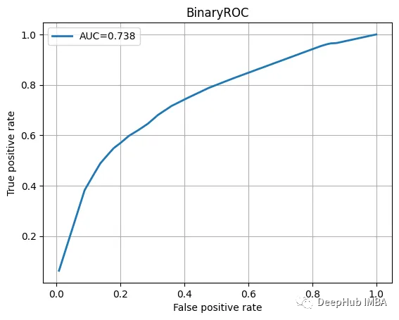
我们训练的模型并不特别复杂,也没有经过精心调整,但它完成了工作。当然这只是一个为了演示使用的小型数据集。
总结
图神经网络尽管看起来很复杂,但是PyTorch Geometric为我们提供了一个很好的解决方案。我们可以直接使用其中内置的模型实现,这方便了我们使用和简化了入门的门槛。
本文代码:https://github.com/maddataanalyst/blogposts_code/blob/main/graph_nns_series/pyg_pyl_perfect_match/pytorch-geometric-lightning-perfect-match.ipynb
The above is the detailed content of Link prediction code example using Pytorch Geometric. For more information, please follow other related articles on the PHP Chinese website!