


Cross-modal Transformer: for fast and robust 3D object detection


Currently, self-driving vehicles have been equipped with a variety of information collection sensors, such as lidar, millimeter-wave radar and camera sensors. From the current point of view, a variety of sensors have shown great development prospects in the perception tasks of autonomous driving. For example, the 2D image information collected by the camera captures rich semantic features, and the point cloud data collected by lidar can provide the accurate position information and geometric information of the object for the perception model. By making full use of the information obtained by different sensors, the occurrence of uncertainty factors in the autonomous driving perception process can be reduced, while the detection robustness of the perception model can be improved.
Today’s introduction is an article from Megvii Autonomous driving perception paper, and was selected for this year's ICCV2023 Vision Summit. The main feature of this article is an End-to-End BEV perception algorithm like PETR (it no longer requires the use of NMS post-processing operations to filter redundant perception results). frame), and at the same time additionally uses the point cloud information of lidar to improve the perception performance of the model. It is a very good paper on the direction of autonomous driving perception. The link to the article and the official open source warehouse link are as follows:
- Paper link: https://arxiv.org/pdf/2301.01283.pdf
- Code link: https://github.com/junjie18/CMT
The overall structure of the CMT algorithm model
Next, we will give an overall introduction to the network structure of the CMT perception model, as shown in the following figure:
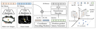
As can be seen from the entire algorithm block diagram, the entire algorithm model mainly consists of three parts
- Lidar backbone network Camera backbone network (Image Backbone Lidar Backbone): used to obtain point clouds and surround images The features are Point Cloud Token**(PC Tokens) and Image Token(Im Tokens)**
- Generation of position coding: For the data information collected by different sensors, Im Tokens generates the corresponding coordinate position code Im PE, PC Tokens generates the corresponding coordinate position code PC PE, and Object QueriesAlso generate the corresponding coordinate position encodingQuery embedding
- Transformer Decoder FFN network: The input is Object Queries Query embedding and complete position encoding Im Tokens and PC Tokens perform cross-attention calculations, and use FFN to generate the final 3D Boxes category prediction
Introduces the overall structure of the network in detail After that, the three sub-parts mentioned above will be introduced in detail
Lidar Backbone Network Camera Backbone Network (Image Backbone Lidar Backbone)
- Lidar Backbone Network
Generally The lidar backbone network used to extract point cloud data features includes the following five parts
- Voxelization of point cloud information
- Voxel feature encoding
- 3D Backbone (commonly used VoxelResBackBone8x network) extracts 3D features from the result of encoding voxel features
- Extract the 3D Backbone to the Z-axis of the feature and compress it to obtain the features in the BEV space
- Use 2D Backbone to perform further feature fitting on the features projected into the BEV space
- Since the number of channels of the feature map output by the 2D Backbone is inconsistent with the number of channels output by the Image, a convolutional layer is used to calculate the number of channels. Alignment (for the model in this article, an alignment of the number of channels is done, but it does not belong to the original point cloud information extraction category)
- Camera backbone network
Generally used cameras The backbone network extracts 2D image features including the following two parts: Input: 16 times and 32 times downsampled feature maps output by the 2D Backbone
Output : Fusion of image features downsampled 16 times and 32 times to obtain feature map downsampled 16 times
Tensor([bs * N, 1024, H / 16 , W/16])Tensor([bs * N, 2048, H/16, W/16])The content that needs to be rewritten is: tensor ([bs * N, 256, H / 16, W / 16])Rewrite content: Use ResNet-50 network to extract features of surround images
Output: Output image features downsampled 16 times and 32 times
Input tensor:
Tensor([bs * N, 3, H, W])Output tensor:
Tensor([bs * N, 1024, H/16, W/16])Output tensor: ``Tensor([bs * N, 2048, H/32, W/32])`
The content that needs to be rewritten is: 2D skeleton extraction image features
Neck (CEFPN)
Generation of position coding
According to the above introduction, the generation of position coding mainly includes three parts, namely image position embedding, point cloud position embedding and query embedding. The following will introduce their generation process one by one
- Image Position Embedding (Im PE)
The generation process of Image Position Embedding is the same as the generation logic of image position encoding in PETR (for details, please refer to PETR The original text of the paper (I won’t elaborate too much here) can be summarized into the following four steps:
- Generate a 3D image frustum point cloud in the image coordinate system
- The 3D image frustum point cloud is transformed into the camera coordinate system using the camera internal parameter matrix to obtain the 3D camera coordinate points
- The 3D points in the camera coordinate system are transformed into the BEV coordinate system using the cam2ego coordinate transformation matrix
- Use the MLP layer to perform position encoding on the converted BEV 3D coordinates to obtain the final image position encoding
- Point Cloud Position Embedding (PC PE)
Point Cloud Position Embedding generation process It can be divided into the following two steps -
Use the
pos2embed()function at the grid coordinate point in the BEV space to embed the two-dimensional horizontal and vertical The coordinate points are transformed into a high-dimensional feature space# 点云位置编码`bev_pos_embeds`的生成bev_pos_embeds = self.bev_embedding(pos2embed(self.coords_bev.to(device), num_pos_feats=self.hidden_dim))def coords_bev(self):x_size, y_size = (grid_size[0] // downsample_scale,grid_size[1] // downsample_scale)meshgrid = [[0, y_size - 1, y_size], [0, x_size - 1, x_size]]batch_y, batch_x = torch.meshgrid(*[torch.linspace(it[0], it[1], it[2]) for it in meshgrid])batch_x = (batch_x + 0.5) / x_sizebatch_y = (batch_y + 0.5) / y_sizecoord_base = torch.cat([batch_x[None], batch_y[None]], dim=0) # 生成BEV网格.coord_base = coord_base.view(2, -1).transpose(1, 0)return coord_base# shape: (x_size *y_size, 2)def pos2embed(pos, num_pos_feats=256, temperature=10000):scale = 2 * math.pipos = pos * scaledim_t = torch.arange(num_pos_feats, dtype=torch.float32, device=pos.device)dim_t = temperature ** (2 * (dim_t // 2) / num_pos_feats)pos_x = pos[..., 0, None] / dim_tpos_y = pos[..., 1, None] / dim_tpos_x = torch.stack((pos_x[..., 0::2].sin(), pos_x[..., 1::2].cos()), dim=-1).flatten(-2)pos_y = torch.stack((pos_y[..., 0::2].sin(), pos_y[..., 1::2].cos()), dim=-1).flatten(-2)posemb = torch.cat((pos_y, pos_x), dim=-1)return posemb# 将二维的x,y坐标编码成512维的高维向量
-
by using a multi-layer perceptron (MLP) network Perform spatial transformation to ensure alignment of channel numbers
-
##Query embedding
In order to make the similarity calculation between Object Queries, Image Token and Lidar Token more accurate, the query embedding in the paper will be generated using the logic of Lidar and Camera generating position encoding; specifically, query embedding = Image Position Embedding ( Same as rv_query_embeds below) Point Cloud Position Embedding (same as bev_query_embeds below).
-
bev_query_embeds generation logic
Because the Object Query in the paper is originally in the BEV space It is initialized, so you can directly reuse the position encoding and bev_embedding() function in the Point Cloud Position Embedding generation logic. The corresponding key code is as follows:def _bev_query_embed(self, ref_points, img_metas):bev_embeds = self.bev_embedding(pos2embed(ref_points, num_pos_feats=self.hidden_dim))return bev_embeds# (bs, Num, 256)
-
rv_query_embeds generation logic needs to be rewritten
In the aforementioned content, Object Query is the initial point in the BEV coordinate system. In order to follow the generation process of Image Position Embedding, the paper needs to first project the 3D space points in the BEV coordinate system to the image coordinate system, and then use the processing logic of the previous generation of Image Position Embedding to ensure that the logic of the generation process is the same. The following is the core code:def _rv_query_embed(self, ref_points, img_metas):pad_h, pad_w = pad_shape# 由归一化坐标点映射回正常的roi range下的3D坐标点ref_points = ref_points * (pc_range[3:] - pc_range[:3]) + pc_range[:3]points = torch.cat([ref_points, ref_points.shape[:-1]], dim=-1)points = bda_mat.inverse().matmul(points)points = points.unsqueeze(1)points = sensor2ego_mats.inverse().matmul(points)points =intrin_mats.matmul(points)proj_points_clone = points.clone() # 选择有效的投影点z_mask = proj_points_clone[..., 2:3, :].detach() > 0proj_points_clone[..., :3, :] = points[..., :3, :] / (points[..., 2:3, :].detach() + z_mask * 1e-6 - (~z_mask) * 1e-6)proj_points_clone = ida_mats.matmul(proj_points_clone)proj_points_clone = proj_points_clone.squeeze(-1)mask = ((proj_points_clone[..., 0] = 0)& (proj_points_clone[..., 1] = 0))mask &= z_mask.view(*mask.shape)coords_d = (1 + torch.arange(depth_num).float() * (pc_range[4] - 1) / depth_num)projback_points = (ida_mats.inverse().matmul(proj_points_clone))projback_points = torch.einsum("bvnc, d -> bvndc", projback_points, coords_d)projback_points = torch.cat([projback_points[..., :3], projback_points.shape[:-1]], dim=-1)projback_points = (sensor2ego_mats.matmul(intrin_mats).matmul(projback_points))projback_points = (bda_mat@ projback_points)projback_points = (projback_points[..., :3] - pc_range[:3]) / (pc_range[3:] - self.pc_range[:3])rv_embeds = self.rv_embedding(projback_points)rv_embeds = (rv_embeds * mask).sum(dim=1)return rv_embedsThrough the above transformation, the process of projecting the points in the BEV space coordinate system to the image coordinate system is completed, and then using the previous processing logic to generate Image Position Embedding to generate rv_query_embeds. Last query embedding = rv_query_embeds bev_query_embeds
Transformer Decoder FFN network
- Transformer Decoder
The calculation logic here is exactly the same as the Decoder in Transformer, but the input data is a little different
- The first point is Memory: the Memory here is the result of Concat between Image Token and Lidar Token (can be understood as the fusion of the two modalities
- The second point is the location Encoding: The position encoding here is the result of concat between rv_query_embeds and bev_query_embeds. query_embed is rv_query_embeds bev_query_embeds;
- FFN network
The function of this FFN network is exactly the same as that in PETR Yes, the specific output results can be found in the original PETR text, so I won’t go into too much detail here.
Experimental results of the paper
First release the CMT For comparative experiments with other autonomous driving perception algorithms, the author of the paper conducted comparisons on the test and val sets of nuScenes respectively. The experimental results are as follows
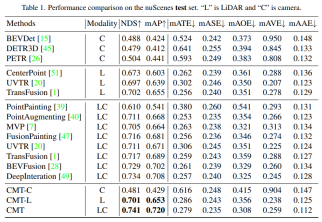
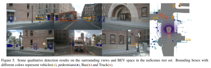
- Comparison of the perception results of each perception algorithm on the test set of nuScenes
Modality in the table represents the sensor category input into the perception algorithm, C represents the camera sensor, and the model only feeds camera data. L represents the lidar sensor, and the model only feeds point cloud data. LC represents lidar and camera sensors , the model inputs multi-modal data. It can be seen from the experimental results that the performance of the CMT-C model is higher than that of BEVDet and DETR3D. The performance of the CMT-L model is higher than that of pure lidar such as CenterPoint and UVTR. Algorithm model. When CMT uses lidar point cloud data and camera data, it surpasses all existing single-modal methods and obtains SOTA results.
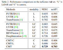
- Comparison of the perception results of the model on the val set of nuScenes
It can be seen from the experimental results that the performance of the CMT-L perception model surpasses FUTR3D and UVTR. When using both lidar point cloud data and After collecting camera data, CMT has greatly surpassed existing multi-modal perception algorithms, such as FUTR3D, UVTR, TransFusion, BEVFusion and other multi-modal algorithms, and achieved SOTA results on val set.
Next is the ablation experiment part of CMT innovation
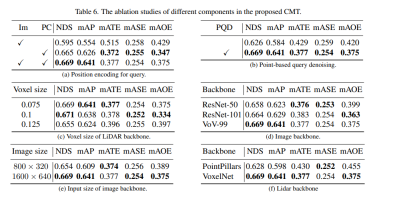
First, we conducted a series of ablation experiments to determine Whether to use positional encoding. Through experimental results, it was found that the NDS and mAP indicators achieve the best results when position encoding of images and lidar is used simultaneously. Next, in parts (c) and (f) of the ablation experiment, we experimented with different types and voxel sizes of the point cloud backbone network. In the ablation experiments in parts (d) and (e), we made different attempts on the type of camera backbone network and the size of the input resolution. The above is just a brief summary of the experimental content. If you want to know more detailed ablation experiments, please refer to the original article
Finally, let’s put a visual display of the CMT perception results on the nuScenes data set. Through the experimental results, you can It can be seen that CMT still has better perception results.
Summary
Currently, fusing various modalities together to improve the perceptual performance of the model has become a popular research Orientation (especially on self-driving cars, equipped with multiple sensors). Meanwhile, CMT is a fully end-to-end perception algorithm that requires no additional post-processing steps and achieves state-of-the-art accuracy on the nuScenes dataset. This article introduces this article in detail, I hope it will be helpful to everyone
The content that needs to be rewritten is: Original link: https://mp.weixin.qq.com/s/Fx7dkv8f2ibkfO66-5hEXA
The above is the detailed content of Cross-modal Transformer: for fast and robust 3D object detection. For more information, please follow other related articles on the PHP Chinese website!

 Gemma Scope: Google's Microscope for Peering into AI's Thought ProcessApr 17, 2025 am 11:55 AM
Exploring the Inner Workings of Language Models with Gemma Scope Understanding the complexities of AI language models is a significant challenge. Google's release of Gemma Scope, a comprehensive toolkit, offers researchers a powerful way to delve in
 Who Is a Business Intelligence Analyst and How To Become One?Apr 17, 2025 am 11:44 AM
Unlocking Business Success: A Guide to Becoming a Business Intelligence Analyst Imagine transforming raw data into actionable insights that drive organizational growth. This is the power of a Business Intelligence (BI) Analyst – a crucial role in gu
 How to Add a Column in SQL? - Analytics VidhyaApr 17, 2025 am 11:43 AM
SQL's ALTER TABLE Statement: Dynamically Adding Columns to Your Database In data management, SQL's adaptability is crucial. Need to adjust your database structure on the fly? The ALTER TABLE statement is your solution. This guide details adding colu
 Business Analyst vs. Data AnalystApr 17, 2025 am 11:38 AM
Introduction Imagine a bustling office where two professionals collaborate on a critical project. The business analyst focuses on the company's objectives, identifying areas for improvement, and ensuring strategic alignment with market trends. Simu
 What are COUNT and COUNTA in Excel? - Analytics VidhyaApr 17, 2025 am 11:34 AM
Excel data counting and analysis: detailed explanation of COUNT and COUNTA functions Accurate data counting and analysis are critical in Excel, especially when working with large data sets. Excel provides a variety of functions to achieve this, with the COUNT and COUNTA functions being key tools for counting the number of cells under different conditions. Although both functions are used to count cells, their design targets are targeted at different data types. Let's dig into the specific details of COUNT and COUNTA functions, highlight their unique features and differences, and learn how to apply them in data analysis. Overview of key points Understand COUNT and COU
 Chrome is Here With AI: Experiencing Something New Everyday!!Apr 17, 2025 am 11:29 AM
Google Chrome's AI Revolution: A Personalized and Efficient Browsing Experience Artificial Intelligence (AI) is rapidly transforming our daily lives, and Google Chrome is leading the charge in the web browsing arena. This article explores the exciti
 AI's Human Side: Wellbeing And The Quadruple Bottom LineApr 17, 2025 am 11:28 AM
Reimagining Impact: The Quadruple Bottom Line For too long, the conversation has been dominated by a narrow view of AI’s impact, primarily focused on the bottom line of profit. However, a more holistic approach recognizes the interconnectedness of bu
 5 Game-Changing Quantum Computing Use Cases You Should Know AboutApr 17, 2025 am 11:24 AM
Things are moving steadily towards that point. The investment pouring into quantum service providers and startups shows that industry understands its significance. And a growing number of real-world use cases are emerging to demonstrate its value out


Hot AI Tools

Undresser.AI Undress
AI-powered app for creating realistic nude photos

AI Clothes Remover
Online AI tool for removing clothes from photos.

Undress AI Tool
Undress images for free

Clothoff.io
AI clothes remover

AI Hentai Generator
Generate AI Hentai for free.

Hot Article
Hot Tools

Zend Studio 13.0.1
Powerful PHP integrated development environment

SublimeText3 English version
Recommended: Win version, supports code prompts!

Dreamweaver CS6
Visual web development tools

MantisBT
Mantis is an easy-to-deploy web-based defect tracking tool designed to aid in product defect tracking. It requires PHP, MySQL and a web server. Check out our demo and hosting services.

VSCode Windows 64-bit Download
A free and powerful IDE editor launched by Microsoft

