
Home >Backend Development >Python Tutorial >Tips | This is probably the best NumPy graphical tutorial I have ever seen!
Tips | This is probably the best NumPy graphical tutorial I have ever seen!

- Python当打之年forward
- 2023-08-10 16:08:121304browse
##In this article, the main usage of NumPy will be introduced, And how it presents different types of data (tables, images, text, etc.), these data processed by Numpy will become the input of the machine learning model.
#Create Array
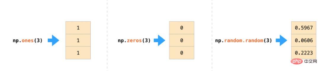
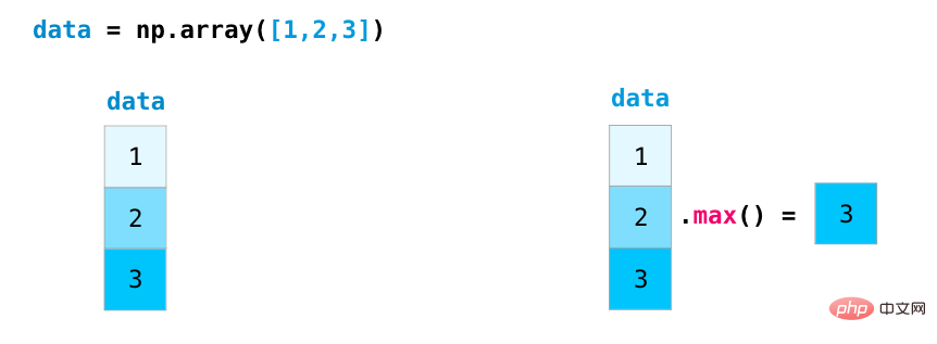
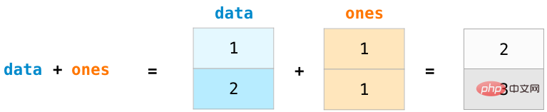
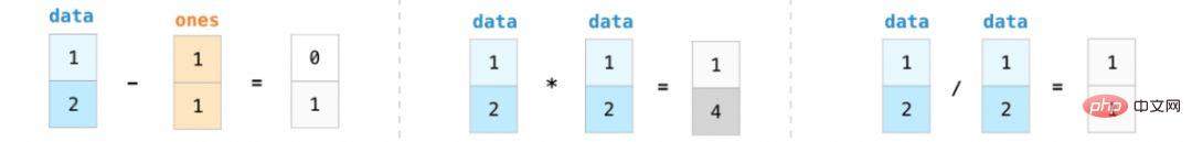
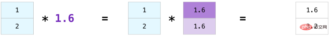
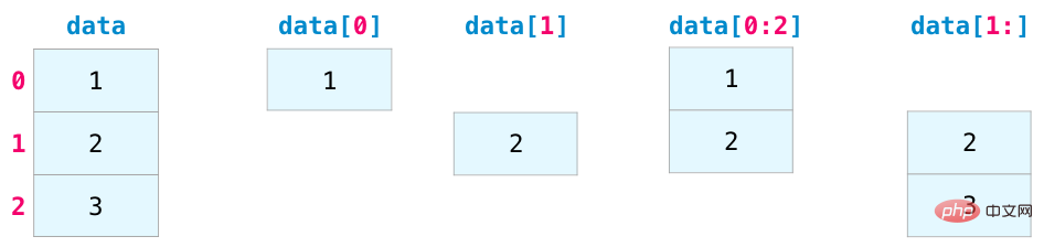
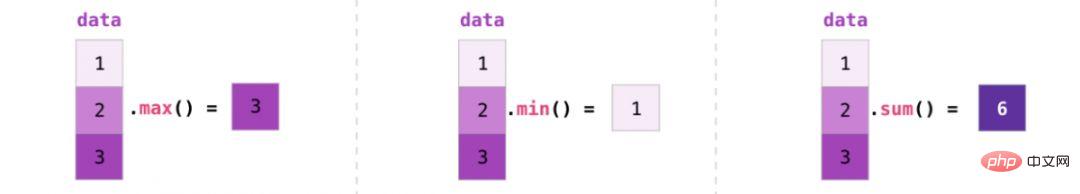
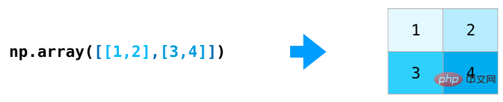
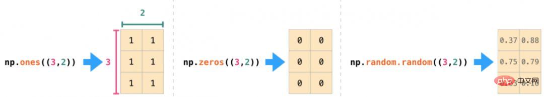
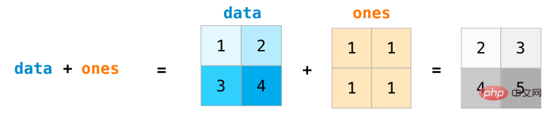
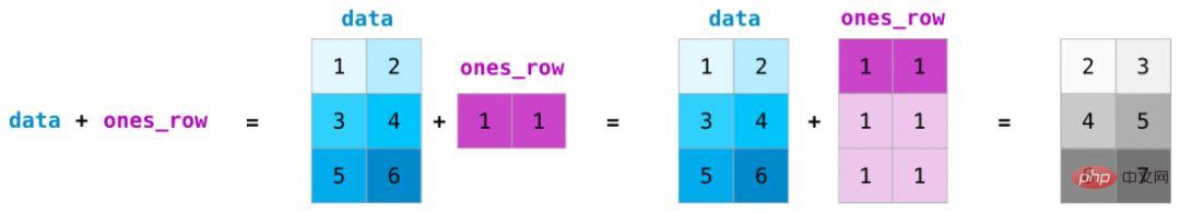
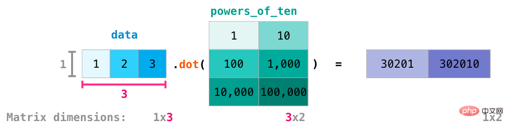
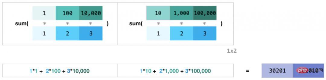
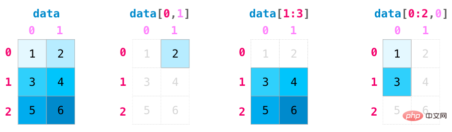
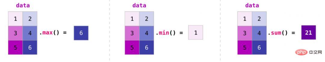
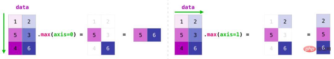
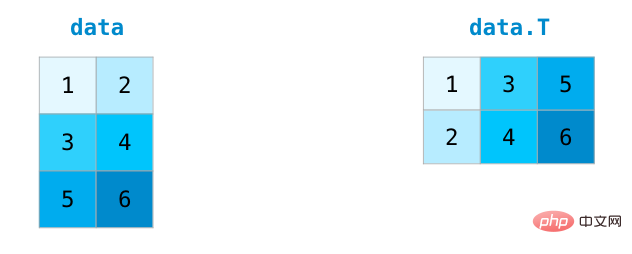
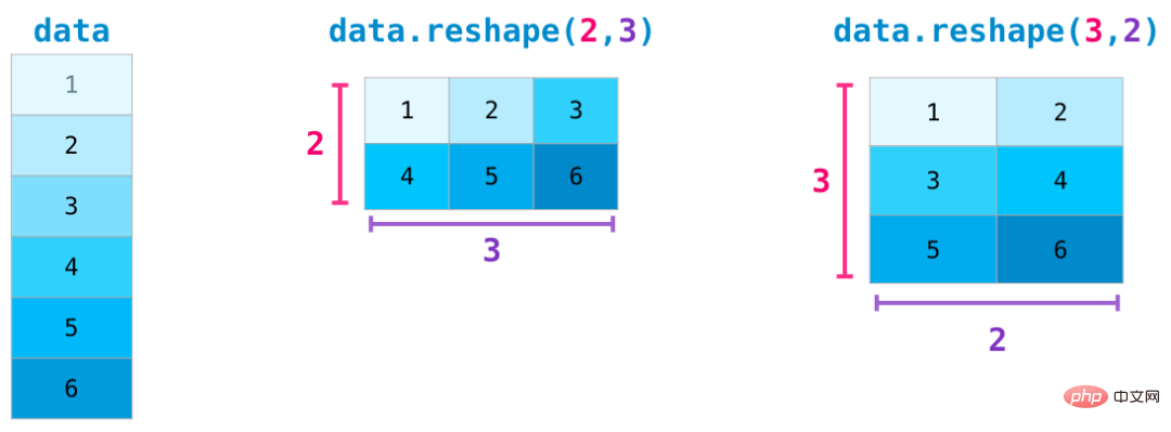
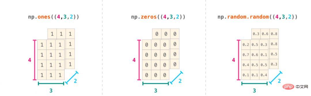
Arithmetic operations on arrays Let us create two NumPy arrays, called For data and ones: ##To calculate two arrays For addition, simply typing data ones can realize the operation of adding the data at the corresponding position (that is, adding each row of data). This operation is more concise than the method code of looping to read the array. In many cases, we want to perform operations on arrays and single values (also known as operations between vectors and scalars). For example: If the array represents distance in miles, our goal is to convert it to kilometers. You can simply write data * 1.6: ##NumPy passes the array Broadcasting knows that this operation requires multiplying each element of the array. Array slicing operation We can index and slice NumPy arrays like python list operations, as shown below: Aggregation function ##The convenience that NumPy brings to us is also the aggregation function, Aggregation functions can compress data and count some feature values in the array: create Matrix We can create a matrix by passing a two-dimensional list to Numpy. np.array([[1,2],[3,4]]) In addition, you can also use ones(), zeros() and random.random() mentioned above to create Matrix, just pass in a tuple to describe the dimensions of the matrix: Arithmetic operations on matrices For two matrices of the same size, we can use the arithmetic operator (-*/) to Add or multiply. NumPy uses position-wise operations for this type of operation: For matrices of different sizes, we can only perform these arithmetic operations when the dimensions of the two matrices are the same as 1 (for example, the matrix has only one column or one row). In this case, NumPy uses the broadcast rule (broadcast ) for operation processing: has a great relationship with arithmetic operations The difference is matrix multiplication using dot product. NumPy provides the dot() method, which can be used to perform dot product operations between matrices: Matrix dimensions have been added at the bottom of the above figure to emphasize that the two matrices being operated on must be equal in columns and rows. This operation can be diagrammed as follows: Slicing and aggregation of matrices Indexing and slicing functions change when manipulating matrices Be more useful. Data can be sliced using index operations on different dimensions. #We can aggregate matrices just like we aggregate vectors: Transposition and reconstruction of matrix When processing matrices, it is often necessary to transpose the matrix. A common situation is to calculate the dot product of two matrices. The property T of a NumPy array can be used to obtain the transpose of a matrix. In more complex use cases, you may find that you need to change The dimensions of a matrix. This is common in machine learning applications, for example, if the input matrix shape of the model is different from the data set, you can use NumPy's reshape() method. Just pass in the new dimensions required for the matrix. You can also pass in -1 and NumPy can infer the correct dimensions based on your matrix:
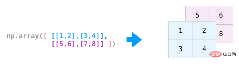
## All the functions above are applicable to multidimensional data, and its central data The structure is called ndarray (N-dimensional array).
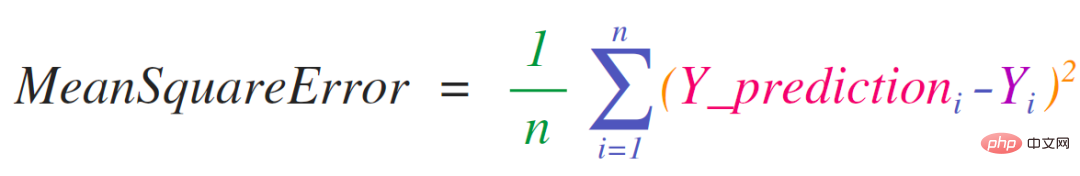
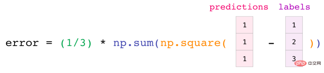
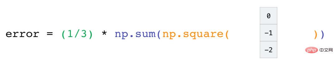
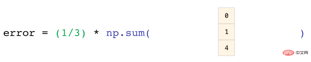
The advantage of this is that numpy does not need to consider the specific values contained in predictions and labels. DigestBacteria will step through the four operations in the above line of code through an example: ##Both the predictions and labels vectors contain three values. This means that the value of n is 3. After we perform the subtraction, we end up with the following values: ##Now we sum these values: Finally get the error value and model quality score of the prediction.
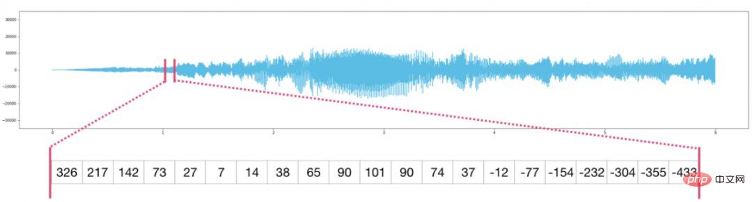
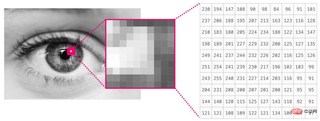
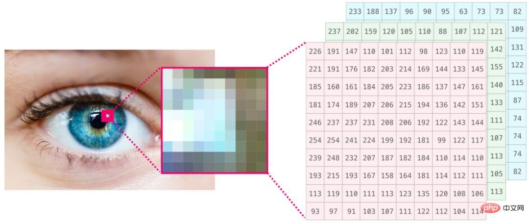
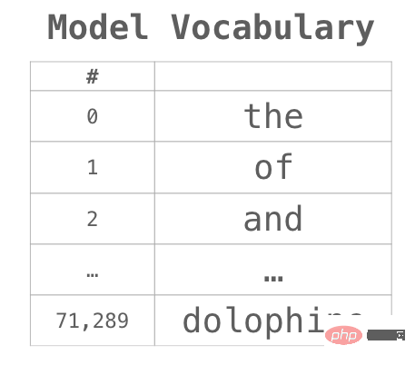
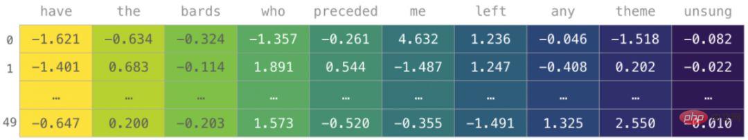
##Audio and Time Series Audio files are one-dimensional arrays of samples. Each sample is a number that represents a small segment of the audio signal. CD-quality audio might have 44,100 samples per second, each sample being an integer between -65535 and 65536. This means that if you have a 10 second CD-quality WAVE file, you can load it into a NumPy array of length 10 * 44,100 = 441,000 samples. Want to extract the first second of audio? Just load the file into a NumPy array we call audio and intercept audio[:44100]. The following is an audio file: The same goes for time series data (for example, a sequence of stock prices over time). Image The image is of size (height × width) pixel matrix. If the image is black and white (also called a grayscale image), each pixel can be represented by a single number (usually between 0 (black) and 255 (white)). If you are processing an image, you can crop a 10 x 10 pixel area in the upper left corner of the image using image[:10,:10] in NumPy. This is a fragment of an image file: #If the image is in color, each pixel is represented by three numbers: red, green, and blue. In this case we need a third dimension (since each cell can only contain one number). So the color image is represented by an ndarray with dimensions (height x width x 3). language If we deal with text, the situation is different. Representing text numerically requires two steps, building a vocabulary (a list of all unique words the model knows) and embedding. Let’s look at the steps to numerically represent this (translated) ancient quote: “Have the bards who preceded me left any theme unsung?” The model needs to be trained on a large amount of text before it can numerically represent the battlefield poet's verses. We can have the model process a small dataset and use this dataset to build a vocabulary (71,290 words): The sentence can then be divided into a series of "word" tokens (words or word parts based on common rules): Then we replace each word with its id from the vocabulary: # These IDs still do not provide valuable information to the model. Therefore, before feeding a sequence of words into the model, the token/word needs to be replaced with an embedding (in this case using a 50-dimensional word2vec embedding): You can see that the dimensions of this NumPy array are [embedding_dimension x sequence_length]. In practice, these values don't necessarily look like this, but I present it this way for visual consistency. For performance reasons, deep learning models tend to retain the first dimension of the batch size (because the model can be trained faster if multiple examples are trained in parallel). Obviously, this is a good place to use reshape(). For example, a model like BERT would expect its input matrix to be of shape: [batch_size, sequence_length, embedding_size]. This is a collection of numbers that the model can process and perform various useful operations. I left many rows blank that can be filled in with additional examples for model training (or prediction). 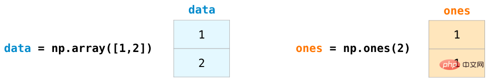
##


##Spreadsheets or data tables are two-dimensional matrices. Each worksheet in the spreadsheet can be its own variable. A similar structure in Python is the pandas dataframe, which is actually built using NumPy. 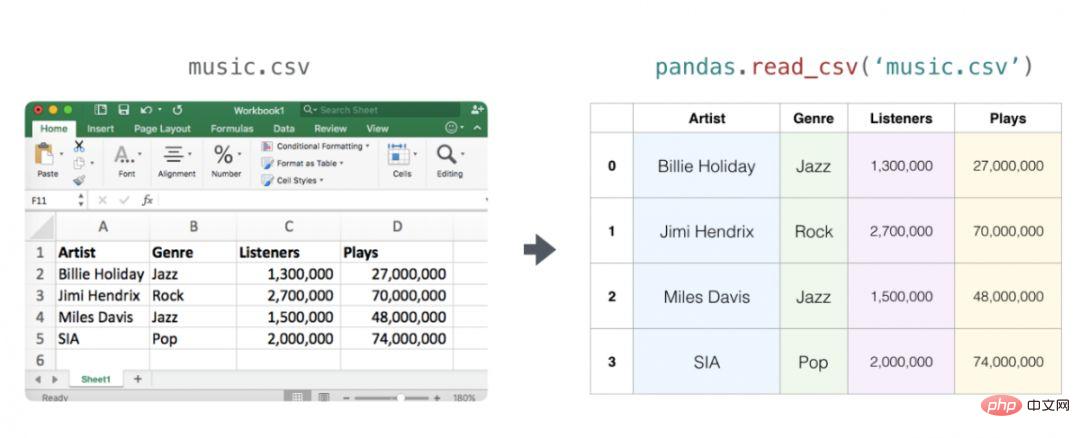


The above is the detailed content of Tips | This is probably the best NumPy graphical tutorial I have ever seen!. For more information, please follow other related articles on the PHP Chinese website!