 Technology peripherals
 AI
AI How to fine-tune LLM with a single GPU to bypass computing power limitations? This is a tutorial on the 'Gradient Accumulation' algorithm
How to fine-tune LLM with a single GPU to bypass computing power limitations? This is a tutorial on the 'Gradient Accumulation' algorithm
Since large models became a hot trend, GPUs have become a scarce commodity. The reserves of many companies may not be sufficient, let alone individual developers. Is there any way to use computing power to train models more efficiently?
In a recent blog, Sebastian Raschka introduced the "gradient accumulation" method, which can use a larger batch size to train the model when GPU memory is limited, bypassing hardware limitations.

Prior to this, Sebastian Raschka also shared an article using a multi-GPU training strategy to accelerate the fine-tuning of large language models. , including mechanisms such as model or tensor sharding, which distribute model weights and computations across different devices to address the memory limitations of GPUs.
Fine-tuning the BLOOM model for classification
Suppose we are interested in adopting a recently pre-trained large language model to handle downstream tasks such as text classification. Then, we might choose to use GPT-3's open source alternative BLOOM model, especially the BLOOM version with "only" 560 million parameters - it should be able to fit into the RAM of a traditional GPU without any problem (Google Colab is free version has a GPU with 15 Gb RAM).
Once you start, you are likely to encounter problems: memory will increase rapidly during training or fine-tuning. The only way to train this model is with a batch size of 1.

The code to fine-tune BLOOM for the target classification task using a batch size of 1 (batch size=1) is as follows. You can also download the complete code on the GitHub project page:
https://github.com/rasbt/gradient-accumulation-blog/blob/main/src/1_batchsize-1.py
You can copy and paste this code directly into Google Colab, but you will also have to drag and drop the accompanying local_dataset_utilities.py file from which some dataset utilities are imported in the same folder.
<code># pip install torch lightning matplotlib pandas torchmetrics watermark transformers datasets -Uimport osimport os.path as opimport timefrom datasets import load_datasetfrom lightning import Fabricimport torchfrom torch.utils.data import DataLoaderimport torchmetricsfrom transformers import AutoTokenizerfrom transformers import AutoModelForSequenceClassificationfrom watermark import watermarkfrom local_dataset_utilities import download_dataset, load_dataset_into_to_dataframe, partition_datasetfrom local_dataset_utilities import IMDBDatasetdef tokenize_text (batch):return tokenizer (batch ["text"], truncatinotallow=True, padding=True, max_length=1024)def train (num_epochs, model, optimizer, train_loader, val_loader, fabric):for epoch in range (num_epochs):train_acc = torchmetrics.Accuracy (task="multiclass", num_classes=2).to (fabric.device)for batch_idx, batch in enumerate (train_loader):model.train ()### FORWARD AND BACK PROPoutputs = model (batch ["input_ids"],attention_mask=batch ["attention_mask"],labels=batch ["label"]) fabric.backward (outputs ["loss"])### UPDATE MODEL PARAMETERSoptimizer.step ()optimizer.zero_grad ()### LOGGINGif not batch_idx % 300:print (f"Epoch: {epoch+1:04d}/{num_epochs:04d}"f"| Batch {batch_idx:04d}/{len (train_loader):04d}"f"| Loss: {outputs ['loss']:.4f}")model.eval ()with torch.no_grad ():predicted_labels = torch.argmax (outputs ["logits"], 1)train_acc.update (predicted_labels, batch ["label"])### MORE LOGGINGmodel.eval ()with torch.no_grad ():val_acc = torchmetrics.Accuracy (task="multiclass", num_classes=2).to (fabric.device)for batch in val_loader:outputs = model (batch ["input_ids"],attention_mask=batch ["attention_mask"],labels=batch ["label"])predicted_labels = torch.argmax (outputs ["logits"], 1)val_acc.update (predicted_labels, batch ["label"])print (f"Epoch: {epoch+1:04d}/{num_epochs:04d}"f"| Train acc.: {train_acc.compute ()*100:.2f}%"f"| Val acc.: {val_acc.compute ()*100:.2f}%")train_acc.reset (), val_acc.reset ()if __name__ == "__main__":print (watermark (packages="torch,lightning,transformers", pythnotallow=True))print ("Torch CUDA available?", torch.cuda.is_available ())device = "cuda" if torch.cuda.is_available () else "cpu"torch.manual_seed (123)# torch.use_deterministic_algorithms (True)############################# 1 Loading the Dataset##########################download_dataset ()df = load_dataset_into_to_dataframe ()if not (op.exists ("train.csv") and op.exists ("val.csv") and op.exists ("test.csv")):partition_dataset (df)imdb_dataset = load_dataset ("csv",data_files={"train": "train.csv","validation": "val.csv","test": "test.csv",},)############################################ 2 Tokenization and Numericalization#########################################tokenizer = AutoTokenizer.from_pretrained ("bigscience/bloom-560m", max_length=1024)print ("Tokenizer input max length:", tokenizer.model_max_length, flush=True)print ("Tokenizer vocabulary size:", tokenizer.vocab_size, flush=True)print ("Tokenizing ...", flush=True)imdb_tokenized = imdb_dataset.map (tokenize_text, batched=True, batch_size=None)del imdb_datasetimdb_tokenized.set_format ("torch", columns=["input_ids", "attention_mask", "label"])os.environ ["TOKENIZERS_PARALLELISM"] = "false"############################################ 3 Set Up DataLoaders#########################################train_dataset = IMDBDataset (imdb_tokenized, partition_key="train")val_dataset = IMDBDataset (imdb_tokenized, partition_key="validation")test_dataset = IMDBDataset (imdb_tokenized, partition_key="test")train_loader = DataLoader (dataset=train_dataset,batch_size=1,shuffle=True,num_workers=4,drop_last=True,)val_loader = DataLoader (dataset=val_dataset,batch_size=1,num_workers=4,drop_last=True,)test_loader = DataLoader (dataset=test_dataset,batch_size=1,num_workers=2,drop_last=True,)############################################ 4 Initializing the Model#########################################fabric = Fabric (accelerator="cuda", devices=1, precisinotallow="16-mixed")fabric.launch ()model = AutoModelForSequenceClassification.from_pretrained ("bigscience/bloom-560m", num_labels=2)optimizer = torch.optim.Adam (model.parameters (), lr=5e-5)model, optimizer = fabric.setup (model, optimizer)train_loader, val_loader, test_loader = fabric.setup_dataloaders (train_loader, val_loader, test_loader)############################################ 5 Finetuning#########################################start = time.time ()train (num_epochs=1,model=model,optimizer=optimizer,train_loader=train_loader,val_loader=val_loader,fabric=fabric,)end = time.time ()elapsed = end-startprint (f"Time elapsed {elapsed/60:.2f} min")with torch.no_grad ():model.eval ()test_acc = torchmetrics.Accuracy (task="multiclass", num_classes=2).to (fabric.device)for batch in test_loader:outputs = model (batch ["input_ids"],attention_mask=batch ["attention_mask"],labels=batch ["label"])predicted_labels = torch.argmax (outputs ["logits"], 1)test_acc.update (predicted_labels, batch ["label"])print (f"Test accuracy {test_acc.compute ()*100:.2f}%")</code>
The author used Lightning Fabric because it gives developers the flexibility to change the number of GPUs and multi-GPU training strategies when running this code on different hardware. It also allows mixed-precision training to be enabled by simply adjusting the precision flag. In this case, mixed-precision training can increase training speed by three times and reduce memory requirements by approximately 25%.
The main code shown above is executed in the main function (if __name__ == "__main__" context). Even if only a single GPU is used, it is recommended to use the PyTorch running environment for execution. Multi-GPU training. Then, the following three code sections contained in if __name__ == "__main__" are responsible for data loading:
# 1 Load the data set
# 2 Tokenization and numericization
# 3 Setting up the data loader
Section 4 is in Initializing the Model , and then in Section 5 Finetuning, the train function is called, which is where things start to get interesting. In the train (...) function, a standard PyTorch loop is implemented. The annotated version of the core training loop looks like this:
The problem with a batch size of 1 (Batch size=1) is that gradient updates will become very confusing and difficult, as shown in the following training The model is based on fluctuating training loss and poor test set performance as seen:
<code>...torch : 2.0.0lightning : 2.0.0transformers: 4.27.2Torch CUDA available? True...Epoch: 0001/0001 | Batch 23700/35000 | Loss: 0.0969Epoch: 0001/0001 | Batch 24000/35000 | Loss: 1.9902Epoch: 0001/0001 | Batch 24300/35000 | Loss: 0.0395Epoch: 0001/0001 | Batch 24600/35000 | Loss: 0.2546Epoch: 0001/0001 | Batch 24900/35000 | Loss: 0.1128Epoch: 0001/0001 | Batch 25200/35000 | Loss: 0.2661Epoch: 0001/0001 | Batch 25500/35000 | Loss: 0.0044Epoch: 0001/0001 | Batch 25800/35000 | Loss: 0.0067Epoch: 0001/0001 | Batch 26100/35000 | Loss: 0.0468Epoch: 0001/0001 | Batch 26400/35000 | Loss: 1.7139Epoch: 0001/0001 | Batch 26700/35000 | Loss: 0.9570Epoch: 0001/0001 | Batch 27000/35000 | Loss: 0.1857Epoch: 0001/0001 | Batch 27300/35000 | Loss: 0.0090Epoch: 0001/0001 | Batch 27600/35000 | Loss: 0.9790Epoch: 0001/0001 | Batch 27900/35000 | Loss: 0.0503Epoch: 0001/0001 | Batch 28200/35000 | Loss: 0.2625Epoch: 0001/0001 | Batch 28500/35000 | Loss: 0.1010Epoch: 0001/0001 | Batch 28800/35000 | Loss: 0.0035Epoch: 0001/0001 | Batch 29100/35000 | Loss: 0.0009Epoch: 0001/0001 | Batch 29400/35000 | Loss: 0.0234Epoch: 0001/0001 | Batch 29700/35000 | Loss: 0.8394Epoch: 0001/0001 | Batch 30000/35000 | Loss: 0.9497Epoch: 0001/0001 | Batch 30300/35000 | Loss: 0.1437Epoch: 0001/0001 | Batch 30600/35000 | Loss: 0.1317Epoch: 0001/0001 | Batch 30900/35000 | Loss: 0.0112Epoch: 0001/0001 | Batch 31200/35000 | Loss: 0.0073Epoch: 0001/0001 | Batch 31500/35000 | Loss: 0.7393Epoch: 0001/0001 | Batch 31800/35000 | Loss: 0.0512Epoch: 0001/0001 | Batch 32100/35000 | Loss: 0.1337Epoch: 0001/0001 | Batch 32400/35000 | Loss: 1.1875Epoch: 0001/0001 | Batch 32700/35000 | Loss: 0.2727Epoch: 0001/0001 | Batch 33000/35000 | Loss: 0.1545Epoch: 0001/0001 | Batch 33300/35000 | Loss: 0.0022Epoch: 0001/0001 | Batch 33600/35000 | Loss: 0.2681Epoch: 0001/0001 | Batch 33900/35000 | Loss: 0.2467Epoch: 0001/0001 | Batch 34200/35000 | Loss: 0.0620Epoch: 0001/0001 | Batch 34500/35000 | Loss: 2.5039Epoch: 0001/0001 | Batch 34800/35000 | Loss: 0.0131Epoch: 0001/0001 | Train acc.: 75.11% | Val acc.: 78.62%Time elapsed 69.97 minTest accuracy 78.53%</code>
Since there are not many GPUs available for tensor sharding, how can it be done? What to train a model with a larger batch size?
One solution is gradient accumulation, which can be used to modify the training loop mentioned earlier.
什么是梯度积累?
梯度累积是一种在训练期间虚拟增加批大小(batch size)的方法,当可用的 GPU 内存不足以容纳所需的批大小时,这非常有用。在梯度累积中,梯度是针对较小的批次计算的,并在多次迭代中累积(通常是求和或平均),而不是在每一批次之后更新模型权重。一旦累积梯度达到目标「虚拟」批大小,模型权重就会使用累积梯度进行更新。
参考下面更新的 PyTorch 训练循环:

如果将 accumulation_steps 设置为 2,那么 zero_grad () 和 optimizer.step () 将只会每隔一秒调用一次。因此,使用 accumulation_steps=2 运行修改后的训练循环与将批大小(batch size)加倍具有相同的效果。
例如,如果想使用 256 的批大小,但只能将 64 的批大小放入 GPU 内存中,就可以对大小为 64 的四个批执行梯度累积。(处理完所有四个批次后,将获得相当于单个批大小为 256 的累积梯度。)这样能够有效地模拟更大的批大小,而无需更大的 GPU 内存或跨不同设备的张量分片。
虽然梯度累积可以帮助我们训练具有更大批量大小的模型,但它不会减少所需的总计算量。实际上,它有时会导致训练过程略慢一些,因为权重更新的执行频率较低。尽管如此,它却能帮我们解决限制问题,即批大小非常小时导致的更新频繁且混乱。
例如,现在让我们运行上面的代码,批大小为 1,需要 16 个累积步骤(accumulation steps)来模拟批大小等于 16。
输出如下:
<code>...torch : 2.0.0lightning : 2.0.0transformers: 4.27.2Torch CUDA available? True...Epoch: 0001/0001 | Batch 23700/35000 | Loss: 0.0168Epoch: 0001/0001 | Batch 24000/35000 | Loss: 0.0006Epoch: 0001/0001 | Batch 24300/35000 | Loss: 0.0152Epoch: 0001/0001 | Batch 24600/35000 | Loss: 0.0003Epoch: 0001/0001 | Batch 24900/35000 | Loss: 0.0623Epoch: 0001/0001 | Batch 25200/35000 | Loss: 0.0010Epoch: 0001/0001 | Batch 25500/35000 | Loss: 0.0001Epoch: 0001/0001 | Batch 25800/35000 | Loss: 0.0047Epoch: 0001/0001 | Batch 26100/35000 | Loss: 0.0004Epoch: 0001/0001 | Batch 26400/35000 | Loss: 0.1016Epoch: 0001/0001 | Batch 26700/35000 | Loss: 0.0021Epoch: 0001/0001 | Batch 27000/35000 | Loss: 0.0015Epoch: 0001/0001 | Batch 27300/35000 | Loss: 0.0008Epoch: 0001/0001 | Batch 27600/35000 | Loss: 0.0060Epoch: 0001/0001 | Batch 27900/35000 | Loss: 0.0001Epoch: 0001/0001 | Batch 28200/35000 | Loss: 0.0426Epoch: 0001/0001 | Batch 28500/35000 | Loss: 0.0012Epoch: 0001/0001 | Batch 28800/35000 | Loss: 0.0025Epoch: 0001/0001 | Batch 29100/35000 | Loss: 0.0025Epoch: 0001/0001 | Batch 29400/35000 | Loss: 0.0000Epoch: 0001/0001 | Batch 29700/35000 | Loss: 0.0495Epoch: 0001/0001 | Batch 30000/35000 | Loss: 0.0164Epoch: 0001/0001 | Batch 30300/35000 | Loss: 0.0067Epoch: 0001/0001 | Batch 30600/35000 | Loss: 0.0037Epoch: 0001/0001 | Batch 30900/35000 | Loss: 0.0005Epoch: 0001/0001 | Batch 31200/35000 | Loss: 0.0013Epoch: 0001/0001 | Batch 31500/35000 | Loss: 0.0112Epoch: 0001/0001 | Batch 31800/35000 | Loss: 0.0053Epoch: 0001/0001 | Batch 32100/35000 | Loss: 0.0012Epoch: 0001/0001 | Batch 32400/35000 | Loss: 0.1365Epoch: 0001/0001 | Batch 32700/35000 | Loss: 0.0210Epoch: 0001/0001 | Batch 33000/35000 | Loss: 0.0374Epoch: 0001/0001 | Batch 33300/35000 | Loss: 0.0007Epoch: 0001/0001 | Batch 33600/35000 | Loss: 0.0341Epoch: 0001/0001 | Batch 33900/35000 | Loss: 0.0259Epoch: 0001/0001 | Batch 34200/35000 | Loss: 0.0005Epoch: 0001/0001 | Batch 34500/35000 | Loss: 0.4792Epoch: 0001/0001 | Batch 34800/35000 | Loss: 0.0003Epoch: 0001/0001 | Train acc.: 78.67% | Val acc.: 87.28%Time elapsed 51.37 minTest accuracy 87.37%</code>
根据上面的结果,损失的波动比以前小了。此外,测试集性能提升了 10%。由于只迭代了训练集一次,因此每个训练样本只会遇到一次。训练用于 multiple epochs 的模型可以进一步提高预测性能。
你可能还会注意到,这段代码的执行速度也比之前使用的批大小为 1 的代码快。如果使用梯度累积将虚拟批大小增加到 8,仍然会有相同数量的前向传播(forward passes)。然而,由于每八个 epoch 只更新一次模型,因此反向传播(backward passes)会很少,这样可更快地在一个 epoch(训练轮数)内迭代样本。
结论
梯度累积是一种在执行权重更新之前通过累积多个小的批梯度来模拟更大的批大小的技术。该技术在可用内存有限且内存中可容纳批大小较小的情况下提供帮助。
但是,首先请思考一种你可以运行批大小的场景,这意味着可用内存大到足以容纳所需的批大小。在那种情况下,梯度累积可能不是必需的。事实上,运行更大的批大小可能更有效,因为它允许更多的并行性且能减少训练模型所需的权重更新次数。
总之,梯度累积是一种实用的技术,可以用于降低小批大小干扰信息对梯度更新准确性的影响。这是迄今一种简单而有效的技术,可以让我们绕过硬件的限制。
PS:可以让这个运行得更快吗?
没问题。可以使用 PyTorch 2.0 中引入的 torch.compile 使其运行得更快。只需要添加一些 model = torch.compile,如下图所示:

GitHub 上提供了完整的脚本。
在这种情况下,torch.compile 在不影响建模性能的情况下又减少了十分钟的训练时间:
<code>poch: 0001/0001 | Batch 26400/35000 | Loss: 0.0320Epoch: 0001/0001 | Batch 26700/35000 | Loss: 0.0010Epoch: 0001/0001 | Batch 27000/35000 | Loss: 0.0006Epoch: 0001/0001 | Batch 27300/35000 | Loss: 0.0015Epoch: 0001/0001 | Batch 27600/35000 | Loss: 0.0157Epoch: 0001/0001 | Batch 27900/35000 | Loss: 0.0015Epoch: 0001/0001 | Batch 28200/35000 | Loss: 0.0540Epoch: 0001/0001 | Batch 28500/35000 | Loss: 0.0035Epoch: 0001/0001 | Batch 28800/35000 | Loss: 0.0016Epoch: 0001/0001 | Batch 29100/35000 | Loss: 0.0015Epoch: 0001/0001 | Batch 29400/35000 | Loss: 0.0008Epoch: 0001/0001 | Batch 29700/35000 | Loss: 0.0877Epoch: 0001/0001 | Batch 30000/35000 | Loss: 0.0232Epoch: 0001/0001 | Batch 30300/35000 | Loss: 0.0014Epoch: 0001/0001 | Batch 30600/35000 | Loss: 0.0032Epoch: 0001/0001 | Batch 30900/35000 | Loss: 0.0004Epoch: 0001/0001 | Batch 31200/35000 | Loss: 0.0062Epoch: 0001/0001 | Batch 31500/35000 | Loss: 0.0032Epoch: 0001/0001 | Batch 31800/35000 | Loss: 0.0066Epoch: 0001/0001 | Batch 32100/35000 | Loss: 0.0017Epoch: 0001/0001 | Batch 32400/35000 | Loss: 0.1485Epoch: 0001/0001 | Batch 32700/35000 | Loss: 0.0324Epoch: 0001/0001 | Batch 33000/35000 | Loss: 0.0155Epoch: 0001/0001 | Batch 33300/35000 | Loss: 0.0007Epoch: 0001/0001 | Batch 33600/35000 | Loss: 0.0049Epoch: 0001/0001 | Batch 33900/35000 | Loss: 0.1170Epoch: 0001/0001 | Batch 34200/35000 | Loss: 0.0002Epoch: 0001/0001 | Batch 34500/35000 | Loss: 0.4201Epoch: 0001/0001 | Batch 34800/35000 | Loss: 0.0018Epoch: 0001/0001 | Train acc.: 78.39% | Val acc.: 86.84%Time elapsed 43.33 minTest accuracy 87.91%</code>
请注意,与之前相比准确率略有提高很可能是由于随机性。

The above is the detailed content of How to fine-tune LLM with a single GPU to bypass computing power limitations? This is a tutorial on the 'Gradient Accumulation' algorithm. For more information, please follow other related articles on the PHP Chinese website!
 Let's Dance: Structured Movement To Fine-Tune Our Human Neural NetsApr 27, 2025 am 11:09 AM
Scientists have extensively studied human and simpler neural networks (like those in C. elegans) to understand their functionality. However, a crucial question arises: how do we adapt our own neural networks to work effectively alongside novel AI s
 New Google Leak Reveals Subscription Changes For Gemini AIApr 27, 2025 am 11:08 AM
Google's Gemini Advanced: New Subscription Tiers on the Horizon Currently, accessing Gemini Advanced requires a $19.99/month Google One AI Premium plan. However, an Android Authority report hints at upcoming changes. Code within the latest Google P
 How Data Analytics Acceleration Is Solving AI's Hidden BottleneckApr 27, 2025 am 11:07 AM
Despite the hype surrounding advanced AI capabilities, a significant challenge lurks within enterprise AI deployments: data processing bottlenecks. While CEOs celebrate AI advancements, engineers grapple with slow query times, overloaded pipelines, a
 MarkItDown MCP Can Convert Any Document into Markdowns!Apr 27, 2025 am 09:47 AM
Handling documents is no longer just about opening files in your AI projects, it’s about transforming chaos into clarity. Docs such as PDFs, PowerPoints, and Word flood our workflows in every shape and size. Retrieving structured
 How to Use Google ADK for Building Agents? - Analytics VidhyaApr 27, 2025 am 09:42 AM
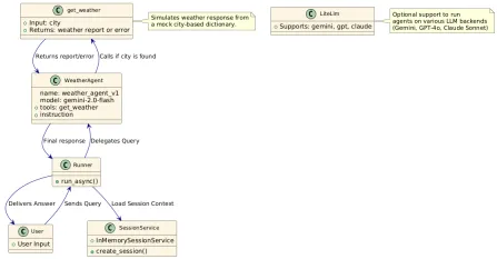
Harness the power of Google's Agent Development Kit (ADK) to create intelligent agents with real-world capabilities! This tutorial guides you through building conversational agents using ADK, supporting various language models like Gemini and GPT. W
 Use of SLM over LLM for Effective Problem Solving - Analytics VidhyaApr 27, 2025 am 09:27 AM
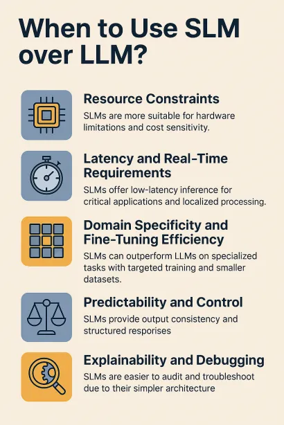
summary: Small Language Model (SLM) is designed for efficiency. They are better than the Large Language Model (LLM) in resource-deficient, real-time and privacy-sensitive environments. Best for focus-based tasks, especially where domain specificity, controllability, and interpretability are more important than general knowledge or creativity. SLMs are not a replacement for LLMs, but they are ideal when precision, speed and cost-effectiveness are critical. Technology helps us achieve more with fewer resources. It has always been a promoter, not a driver. From the steam engine era to the Internet bubble era, the power of technology lies in the extent to which it helps us solve problems. Artificial intelligence (AI) and more recently generative AI are no exception
 How to Use Google Gemini Models for Computer Vision Tasks? - Analytics VidhyaApr 27, 2025 am 09:26 AM
Harness the Power of Google Gemini for Computer Vision: A Comprehensive Guide Google Gemini, a leading AI chatbot, extends its capabilities beyond conversation to encompass powerful computer vision functionalities. This guide details how to utilize
 Gemini 2.0 Flash vs o4-mini: Can Google Do Better Than OpenAI?Apr 27, 2025 am 09:20 AM
The AI landscape of 2025 is electrifying with the arrival of Google's Gemini 2.0 Flash and OpenAI's o4-mini. These cutting-edge models, launched weeks apart, boast comparable advanced features and impressive benchmark scores. This in-depth compariso


Hot AI Tools

Undresser.AI Undress
AI-powered app for creating realistic nude photos

AI Clothes Remover
Online AI tool for removing clothes from photos.

Undress AI Tool
Undress images for free

Clothoff.io
AI clothes remover

Video Face Swap
Swap faces in any video effortlessly with our completely free AI face swap tool!

Hot Article

Hot Tools

PhpStorm Mac version
The latest (2018.2.1) professional PHP integrated development tool

MinGW - Minimalist GNU for Windows
This project is in the process of being migrated to osdn.net/projects/mingw, you can continue to follow us there. MinGW: A native Windows port of the GNU Compiler Collection (GCC), freely distributable import libraries and header files for building native Windows applications; includes extensions to the MSVC runtime to support C99 functionality. All MinGW software can run on 64-bit Windows platforms.

EditPlus Chinese cracked version
Small size, syntax highlighting, does not support code prompt function

DVWA
Damn Vulnerable Web App (DVWA) is a PHP/MySQL web application that is very vulnerable. Its main goals are to be an aid for security professionals to test their skills and tools in a legal environment, to help web developers better understand the process of securing web applications, and to help teachers/students teach/learn in a classroom environment Web application security. The goal of DVWA is to practice some of the most common web vulnerabilities through a simple and straightforward interface, with varying degrees of difficulty. Please note that this software

ZendStudio 13.5.1 Mac
Powerful PHP integrated development environment


