How to realize monocular 3D reconstruction based on python

1. Overview of monocular 3D reconstruction

Although the objects in the objective world are three-dimensional, the images we obtain are two-dimensional, but we can The three-dimensional information of the target is sensed in these two-dimensional images. Three-dimensional reconstruction technology processes images in a certain way to obtain three-dimensional information that can be recognized by computers, thereby analyzing the target. Monocular 3D reconstruction simulates binocular vision based on the movement of a single camera to obtain three-dimensional visual information of objects in space, where monocular refers to a single camera.

2. Implementation process

In the process of monocular three-dimensional reconstruction of objects, the relevant operating environment is as follows:

matplotlib 3.3.4
numpy 1.19.5
opencv-contrib-python 3.4.2.16
opencv-python 3.4.2.16
pillow 8.2.0
python 3.6.2

The reconstruction mainly includes The following steps:

(1) Camera calibration

(2) Image feature extraction and matching

(3) Three-dimensional reconstruction

Next, we Let’s take a detailed look at the specific implementation of each step:

(1) Camera calibration

There are many cameras in our daily lives, such as cameras on mobile phones, digital cameras and functional module types. Cameras, etc. The parameters of each camera are different, that is, the resolution, mode, etc. of the photos taken by the camera. Assuming that when we perform three-dimensional reconstruction of an object, we do not know the matrix parameters of our camera in advance, then we should calculate the matrix parameters of the camera. This step is called camera calibration. I won’t introduce the relevant principles of camera calibration. Many people on the Internet have explained it in detail. The specific implementation of the calibration is as follows:

def camera_calibration(ImagePath):
    # 循环中断
    criteria = (cv2.TERM_CRITERIA_EPS + cv2.TERM_CRITERIA_MAX_ITER, 30, 0.001)
    # 棋盘格尺寸（棋盘格的交叉点的个数）
    row = 11
    column = 8
    
    objpoint = np.zeros((row * column, 3), np.float32)
    objpoint[:, :2] = np.mgrid[0:row, 0:column].T.reshape(-1, 2)

    objpoints = []  # 3d point in real world space
    imgpoints = []  # 2d points in image plane.

    batch_images = glob.glob(ImagePath + '/*.jpg')
    for i, fname in enumerate(batch_images):
        img = cv2.imread(batch_images[i])
        imgGray = cv2.cvtColor(img, cv2.COLOR_BGR2GRAY)
        # find chess board corners
        ret, corners = cv2.findChessboardCorners(imgGray, (row, column), None)
        # if found, add object points, image points (after refining them)
        if ret:
            objpoints.append(objpoint)
            corners2 = cv2.cornerSubPix(imgGray, corners, (11, 11), (-1, -1), criteria)
            imgpoints.append(corners2)
            # Draw and display the corners
            img = cv2.drawChessboardCorners(img, (row, column), corners2, ret)
            cv2.imwrite('Checkerboard_Image/Temp_JPG/Temp_' + str(i) + '.jpg', img)

    print("成功提取:", len(batch_images), "张图片角点！")
    ret, mtx, dist, rvecs, tvecs = cv2.calibrateCamera(objpoints, imgpoints, imgGray.shape[::-1], None, None)

Among them, the mtx matrix obtained by the cv2.calibrateCamera function is the K matrix.

After modifying the corresponding parameters and completing the calibration, we can output the corner point image of the checkerboard to see whether the corner points of the checkerboard have been successfully extracted. The output corner point image is as follows:

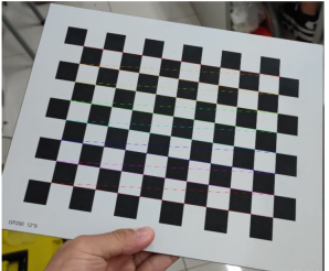
Figure 1: Checkerboard corner point extraction

(2) Image feature extraction and matching

In the entire three-dimensional reconstruction process, this step is the most critical It is also the most complicated step. The quality of image feature extraction determines your final reconstruction effect.
Among the image feature point extraction algorithms, there are three commonly used algorithms, namely: SIFT algorithm, SURF algorithm and ORB algorithm. Through comprehensive analysis and comparison, we use the SURF algorithm to extract the feature points of the image in this step. If you are interested in comparing the feature point extraction effects of the three algorithms, you can search online and have a look. I will not compare them one by one here. The specific implementation is as follows:

def epipolar_geometric(Images_Path, K):
    IMG = glob.glob(Images_Path)
    img1, img2 = cv2.imread(IMG[0]), cv2.imread(IMG[1])
    img1_gray = cv2.cvtColor(img1, cv2.COLOR_BGR2GRAY)
    img2_gray = cv2.cvtColor(img2, cv2.COLOR_BGR2GRAY)

    # Initiate SURF detector
    SURF = cv2.xfeatures2d_SURF.create()

    # compute keypoint & descriptions
    keypoint1, descriptor1 = SURF.detectAndCompute(img1_gray, None)
    keypoint2, descriptor2 = SURF.detectAndCompute(img2_gray, None)
    print("角点数量：", len(keypoint1), len(keypoint2))

    # Find point matches
    bf = cv2.BFMatcher(cv2.NORM_L2, crossCheck=True)
    matches = bf.match(descriptor1, descriptor2)
    print("匹配点数量：", len(matches))

    src_pts = np.asarray([keypoint1[m.queryIdx].pt for m in matches])
    dst_pts = np.asarray([keypoint2[m.trainIdx].pt for m in matches])
    # plot
    knn_image = cv2.drawMatches(img1_gray, keypoint1, img2_gray, keypoint2, matches[:-1], None, flags=2)
    image_ = Image.fromarray(np.uint8(knn_image))
    image_.save("MatchesImage.jpg")

    # Constrain matches to fit homography
    retval, mask = cv2.findHomography(src_pts, dst_pts, cv2.RANSAC, 100.0)

    # We select only inlier points
    points1 = src_pts[mask.ravel() == 1]
    points2 = dst_pts[mask.ravel() == 1]

The found feature points are as follows:

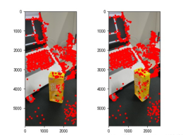
Figure 2: Feature point extraction

(3) Three-dimensional reconstruction

After we find the feature points of the image and match each other, we can start the three-dimensional reconstruction. The specific implementation is as follows:

points1 = cart2hom(points1.T)
points2 = cart2hom(points2.T)
# plot
fig, ax = plt.subplots(1, 2)
ax[0].autoscale_view('tight')
ax[0].imshow(cv2.cvtColor(img1, cv2.COLOR_BGR2RGB))
ax[0].plot(points1[0], points1[1], 'r.')
ax[1].autoscale_view('tight')
ax[1].imshow(cv2.cvtColor(img2, cv2.COLOR_BGR2RGB))
ax[1].plot(points2[0], points2[1], 'r.')
plt.savefig('MatchesPoints.jpg')
fig.show()
# 

points1n = np.dot(np.linalg.inv(K), points1)
points2n = np.dot(np.linalg.inv(K), points2)
E = compute_essential_normalized(points1n, points2n)
print('Computed essential matrix:', (-E / E[0][1]))

P1 = np.array([[1, 0, 0, 0], [0, 1, 0, 0], [0, 0, 1, 0]])
P2s = compute_P_from_essential(E)

ind = -1
for i, P2 in enumerate(P2s):
    # Find the correct camera parameters
    d1 = reconstruct_one_point(points1n[:, 0], points2n[:, 0], P1, P2)
    # Convert P2 from camera view to world view
    P2_homogenous = np.linalg.inv(np.vstack([P2, [0, 0, 0, 1]]))
    d2 = np.dot(P2_homogenous[:3, :4], d1)
    if d1[2] > 0 and d2[2] > 0:
        ind = i

P2 = np.linalg.inv(np.vstack([P2s[ind], [0, 0, 0, 1]]))[:3, :4]
Points3D = linear_triangulation(points1n, points2n, P1, P2)

fig = plt.figure()
fig.suptitle('3D reconstructed', fontsize=16)
ax = fig.gca(projection='3d')
ax.plot(Points3D[0], Points3D[1], Points3D[2], 'b.')
ax.set_xlabel('x axis')
ax.set_ylabel('y axis')
ax.set_zlabel('z axis')
ax.view_init(elev=135, azim=90)
plt.savefig('Reconstruction.jpg')
plt.show()

The reconstruction effect is as follows (the effect is average):

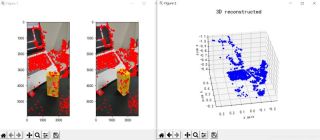
Figure 3: Three-dimensional reconstruction

3. Conclusion

From the reconstruction results, the monocular three-dimensional reconstruction effect is average. I think it may be related to these aspects. Related factors:

(1) Picture shooting form. If it is a monocular three-dimensional reconstruction task, it is best to keep moving the camera parallel when taking pictures, and it is best to take pictures from the front, that is, do not take pictures at an angle or at a special angle;

(2) Surrounding environment when shooting interference. It is best to choose a single shooting location to reduce interference from irrelevant objects;

(3) Shooting light source problem. The chosen photo location must ensure appropriate brightness (you will need to test the specific situation to know whether your light source meets the standard), and when moving the camera, you must also ensure that the light source is consistent between the previous moment and this moment.

In fact, the performance of monocular 3D reconstruction is usually poor. Even when all conditions are optimal, the resulting reconstruction effect is not very good. Or we can consider using binocular 3D reconstruction. The effect of binocular 3D reconstruction is definitely better than the effect of monocular, and the implementation is only a little bit troublesome, haha. In fact, the operation is not complicated. The most troublesome part is shooting and calibrating the two cameras. Other aspects are relatively easy.

4. Code

import cv2
import json
import numpy as np
import glob
from PIL import Image
import matplotlib.pyplot as plt
plt.rcParams['font.sans-serif'] = ['SimHei']
plt.rcParams['axes.unicode_minus'] = False


def cart2hom(arr):
    """ Convert catesian to homogenous points by appending a row of 1s
    :param arr: array of shape (num_dimension x num_points)
    :returns: array of shape ((num_dimension+1) x num_points) 
    """
    if arr.ndim == 1:
        return np.hstack([arr, 1])
    return np.asarray(np.vstack([arr, np.ones(arr.shape[1])]))


def compute_P_from_essential(E):
    """ Compute the second camera matrix (assuming P1 = [I 0])
        from an essential matrix. E = [t]R
    :returns: list of 4 possible camera matrices.
    """
    U, S, V = np.linalg.svd(E)

    # Ensure rotation matrix are right-handed with positive determinant
    if np.linalg.det(np.dot(U, V)) < 0:
        V = -V

    # create 4 possible camera matrices (Hartley p 258)
    W = np.array([[0, -1, 0], [1, 0, 0], [0, 0, 1]])
    P2s = [np.vstack((np.dot(U, np.dot(W, V)).T, U[:, 2])).T,
           np.vstack((np.dot(U, np.dot(W, V)).T, -U[:, 2])).T,
           np.vstack((np.dot(U, np.dot(W.T, V)).T, U[:, 2])).T,
           np.vstack((np.dot(U, np.dot(W.T, V)).T, -U[:, 2])).T]

    return P2s


def correspondence_matrix(p1, p2):
    p1x, p1y = p1[:2]
    p2x, p2y = p2[:2]

    return np.array([
        p1x * p2x, p1x * p2y, p1x,
        p1y * p2x, p1y * p2y, p1y,
        p2x, p2y, np.ones(len(p1x))
    ]).T

    return np.array([
        p2x * p1x, p2x * p1y, p2x,
        p2y * p1x, p2y * p1y, p2y,
        p1x, p1y, np.ones(len(p1x))
    ]).T


def scale_and_translate_points(points):
    """ Scale and translate image points so that centroid of the points
        are at the origin and avg distance to the origin is equal to sqrt(2).
    :param points: array of homogenous point (3 x n)
    :returns: array of same input shape and its normalization matrix
    """
    x = points[0]
    y = points[1]
    center = points.mean(axis=1)  # mean of each row
    cx = x - center[0]  # center the points
    cy = y - center[1]
    dist = np.sqrt(np.power(cx, 2) + np.power(cy, 2))
    scale = np.sqrt(2) / dist.mean()
    norm3d = np.array([
        [scale, 0, -scale * center[0]],
        [0, scale, -scale * center[1]],
        [0, 0, 1]
    ])

    return np.dot(norm3d, points), norm3d


def compute_image_to_image_matrix(x1, x2, compute_essential=False):
    """ Compute the fundamental or essential matrix from corresponding points
        (x1, x2 3*n arrays) using the 8 point algorithm.
        Each row in the A matrix below is constructed as
        [x'*x, x'*y, x', y'*x, y'*y, y', x, y, 1]
    """
    A = correspondence_matrix(x1, x2)
    # compute linear least square solution
    U, S, V = np.linalg.svd(A)
    F = V[-1].reshape(3, 3)

    # constrain F. Make rank 2 by zeroing out last singular value
    U, S, V = np.linalg.svd(F)
    S[-1] = 0
    if compute_essential:
        S = [1, 1, 0]  # Force rank 2 and equal eigenvalues
    F = np.dot(U, np.dot(np.diag(S), V))

    return F


def compute_normalized_image_to_image_matrix(p1, p2, compute_essential=False):
    """ Computes the fundamental or essential matrix from corresponding points
        using the normalized 8 point algorithm.
    :input p1, p2: corresponding points with shape 3 x n
    :returns: fundamental or essential matrix with shape 3 x 3
    """
    n = p1.shape[1]
    if p2.shape[1] != n:
        raise ValueError('Number of points do not match.')

    # preprocess image coordinates
    p1n, T1 = scale_and_translate_points(p1)
    p2n, T2 = scale_and_translate_points(p2)

    # compute F or E with the coordinates
    F = compute_image_to_image_matrix(p1n, p2n, compute_essential)

    # reverse preprocessing of coordinates
    # We know that P1' E P2 = 0
    F = np.dot(T1.T, np.dot(F, T2))

    return F / F[2, 2]


def compute_fundamental_normalized(p1, p2):
    return compute_normalized_image_to_image_matrix(p1, p2)


def compute_essential_normalized(p1, p2):
    return compute_normalized_image_to_image_matrix(p1, p2, compute_essential=True)


def skew(x):
    """ Create a skew symmetric matrix *A* from a 3d vector *x*.
        Property: np.cross(A, v) == np.dot(x, v)
    :param x: 3d vector
    :returns: 3 x 3 skew symmetric matrix from *x*
    """
    return np.array([
        [0, -x[2], x[1]],
        [x[2], 0, -x[0]],
        [-x[1], x[0], 0]
    ])


def reconstruct_one_point(pt1, pt2, m1, m2):
    """
        pt1 and m1 * X are parallel and cross product = 0
        pt1 x m1 * X  =  pt2 x m2 * X  =  0
    """
    A = np.vstack([
        np.dot(skew(pt1), m1),
        np.dot(skew(pt2), m2)
    ])
    U, S, V = np.linalg.svd(A)
    P = np.ravel(V[-1, :4])

    return P / P[3]


def linear_triangulation(p1, p2, m1, m2):
    """
    Linear triangulation (Hartley ch 12.2 pg 312) to find the 3D point X
    where p1 = m1 * X and p2 = m2 * X. Solve AX = 0.
    :param p1, p2: 2D points in homo. or catesian coordinates. Shape (3 x n)
    :param m1, m2: Camera matrices associated with p1 and p2. Shape (3 x 4)
    :returns: 4 x n homogenous 3d triangulated points
    """
    num_points = p1.shape[1]
    res = np.ones((4, num_points))

    for i in range(num_points):
        A = np.asarray([
            (p1[0, i] * m1[2, :] - m1[0, :]),
            (p1[1, i] * m1[2, :] - m1[1, :]),
            (p2[0, i] * m2[2, :] - m2[0, :]),
            (p2[1, i] * m2[2, :] - m2[1, :])
        ])

        _, _, V = np.linalg.svd(A)
        X = V[-1, :4]
        res[:, i] = X / X[3]

    return res


def writetofile(dict, path):
    for index, item in enumerate(dict):
        dict[item] = np.array(dict[item])
        dict[item] = dict[item].tolist()
    js = json.dumps(dict)
    with open(path, 'w') as f:
        f.write(js)
        print("参数已成功保存到文件")


def readfromfile(path):
    with open(path, 'r') as f:
        js = f.read()
        mydict = json.loads(js)
    print("参数读取成功")
    return mydict


def camera_calibration(SaveParamPath, ImagePath):
    # 循环中断
    criteria = (cv2.TERM_CRITERIA_EPS + cv2.TERM_CRITERIA_MAX_ITER, 30, 0.001)
    # 棋盘格尺寸
    row = 11
    column = 8
    objpoint = np.zeros((row * column, 3), np.float32)
    objpoint[:, :2] = np.mgrid[0:row, 0:column].T.reshape(-1, 2)

    objpoints = []  # 3d point in real world space
    imgpoints = []  # 2d points in image plane.
    batch_images = glob.glob(ImagePath + '/*.jpg')
    for i, fname in enumerate(batch_images):
        img = cv2.imread(batch_images[i])
        imgGray = cv2.cvtColor(img, cv2.COLOR_BGR2GRAY)
        # find chess board corners
        ret, corners = cv2.findChessboardCorners(imgGray, (row, column), None)
        # if found, add object points, image points (after refining them)
        if ret:
            objpoints.append(objpoint)
            corners2 = cv2.cornerSubPix(imgGray, corners, (11, 11), (-1, -1), criteria)
            imgpoints.append(corners2)
            # Draw and display the corners
            img = cv2.drawChessboardCorners(img, (row, column), corners2, ret)
            cv2.imwrite('Checkerboard_Image/Temp_JPG/Temp_' + str(i) + '.jpg', img)
    print("成功提取:", len(batch_images), "张图片角点！")
    ret, mtx, dist, rvecs, tvecs = cv2.calibrateCamera(objpoints, imgpoints, imgGray.shape[::-1], None, None)
    dict = {'ret': ret, 'mtx': mtx, 'dist': dist, 'rvecs': rvecs, 'tvecs': tvecs}
    writetofile(dict, SaveParamPath)

    meanError = 0
    for i in range(len(objpoints)):
        imgpoints2, _ = cv2.projectPoints(objpoints[i], rvecs[i], tvecs[i], mtx, dist)
        error = cv2.norm(imgpoints[i], imgpoints2, cv2.NORM_L2) / len(imgpoints2)
        meanError += error
    print("total error: ", meanError / len(objpoints))


def epipolar_geometric(Images_Path, K):
    IMG = glob.glob(Images_Path)
    img1, img2 = cv2.imread(IMG[0]), cv2.imread(IMG[1])
    img1_gray = cv2.cvtColor(img1, cv2.COLOR_BGR2GRAY)
    img2_gray = cv2.cvtColor(img2, cv2.COLOR_BGR2GRAY)

    # Initiate SURF detector
    SURF = cv2.xfeatures2d_SURF.create()

    # compute keypoint & descriptions
    keypoint1, descriptor1 = SURF.detectAndCompute(img1_gray, None)
    keypoint2, descriptor2 = SURF.detectAndCompute(img2_gray, None)
    print("角点数量：", len(keypoint1), len(keypoint2))

    # Find point matches
    bf = cv2.BFMatcher(cv2.NORM_L2, crossCheck=True)
    matches = bf.match(descriptor1, descriptor2)
    print("匹配点数量：", len(matches))

    src_pts = np.asarray([keypoint1[m.queryIdx].pt for m in matches])
    dst_pts = np.asarray([keypoint2[m.trainIdx].pt for m in matches])
    # plot
    knn_image = cv2.drawMatches(img1_gray, keypoint1, img2_gray, keypoint2, matches[:-1], None, flags=2)
    image_ = Image.fromarray(np.uint8(knn_image))
    image_.save("MatchesImage.jpg")

    # Constrain matches to fit homography
    retval, mask = cv2.findHomography(src_pts, dst_pts, cv2.RANSAC, 100.0)

    # We select only inlier points
    points1 = src_pts[mask.ravel() == 1]
    points2 = dst_pts[mask.ravel() == 1]

    points1 = cart2hom(points1.T)
    points2 = cart2hom(points2.T)
    # plot
    fig, ax = plt.subplots(1, 2)
    ax[0].autoscale_view('tight')
    ax[0].imshow(cv2.cvtColor(img1, cv2.COLOR_BGR2RGB))
    ax[0].plot(points1[0], points1[1], 'r.')
    ax[1].autoscale_view('tight')
    ax[1].imshow(cv2.cvtColor(img2, cv2.COLOR_BGR2RGB))
    ax[1].plot(points2[0], points2[1], 'r.')
    plt.savefig('MatchesPoints.jpg')
    fig.show()
    # 

    points1n = np.dot(np.linalg.inv(K), points1)
    points2n = np.dot(np.linalg.inv(K), points2)
    E = compute_essential_normalized(points1n, points2n)
    print('Computed essential matrix:', (-E / E[0][1]))

    P1 = np.array([[1, 0, 0, 0], [0, 1, 0, 0], [0, 0, 1, 0]])
    P2s = compute_P_from_essential(E)

    ind = -1
    for i, P2 in enumerate(P2s):
        # Find the correct camera parameters
        d1 = reconstruct_one_point(points1n[:, 0], points2n[:, 0], P1, P2)
        # Convert P2 from camera view to world view
        P2_homogenous = np.linalg.inv(np.vstack([P2, [0, 0, 0, 1]]))
        d2 = np.dot(P2_homogenous[:3, :4], d1)
        if d1[2] > 0 and d2[2] > 0:
            ind = i

    P2 = np.linalg.inv(np.vstack([P2s[ind], [0, 0, 0, 1]]))[:3, :4]
    Points3D = linear_triangulation(points1n, points2n, P1, P2)

    return Points3D


def main():
    CameraParam_Path = 'CameraParam.txt'
    CheckerboardImage_Path = 'Checkerboard_Image'
    Images_Path = 'SubstitutionCalibration_Image/*.jpg'

    # 计算相机参数
    camera_calibration(CameraParam_Path, CheckerboardImage_Path)
    # 读取相机参数
    config = readfromfile(CameraParam_Path)
    K = np.array(config['mtx'])
    # 计算3D点
    Points3D = epipolar_geometric(Images_Path, K)
    # 重建3D点
    fig = plt.figure()
    fig.suptitle('3D reconstructed', fontsize=16)
    ax = fig.gca(projection='3d')
    ax.plot(Points3D[0], Points3D[1], Points3D[2], 'b.')
    ax.set_xlabel('x axis')
    ax.set_ylabel('y axis')
    ax.set_zlabel('z axis')
    ax.view_init(elev=135, azim=90)
    plt.savefig('Reconstruction.jpg')
    plt.show()


if __name__ == '__main__':
    main()

The above is the detailed content of How to realize monocular 3D reconstruction based on python. For more information, please follow other related articles on the PHP Chinese website!