 Technology peripherals
 AI
AI Setting the best threshold for machine learning models: Is 0.5 the best threshold for binary classification?
Setting the best threshold for machine learning models: Is 0.5 the best threshold for binary classification?
For binary classification, the classifier outputs a real-valued score, and then generates a binary response by thresholding the value. For example, logistic regression outputs a probability (a value between 0.0 and 1.0); observations with scores equal to or above 0.5 produce a positive output (many other models use a 0.5 threshold by default).
But using the default 0.5 threshold is not ideal. In this article I will show how to choose the best threshold from a binary classifier. This article will use Plomber to execute our experiments in parallel and use sklearn-evaluation to generate graphs.

Here is an example of training logistic regression. Suppose we are developing a content moderation system, where the model flags posts containing harmful content (images, videos, etc.); a human then looks at it and decides whether the content should be removed.
Build a simple binary classifier
The following code snippet trains our classifier:
import matplotlib.pyplot as plt
 import matplotlib as mpl
 from sklearn import datasets
 from sklearn.linear_model import LogisticRegression
 from sklearn.model_selection import train_test_split
 from sklearn_evaluation.plot import ConfusionMatrix

 # matplotlib settings
 mpl.rcParams['figure.figsize'] = (4, 4)
 mpl.rcParams['figure.dpi'] = 150

 # create sample dataset
 X, y = datasets.make_classification(1000, 10, n_informative=5, class_sep=0.4)
 X_train, X_test, y_train, y_test = train_test_split(X, y, test_size=0.3)

 # fit model
 clf = LogisticRegression()
 _ = clf.fit(X_train, y_train)
Now let us make predictions on the test set and evaluate it through the confusion matrix Performance:
# predict on the test set
 y_pred = clf.predict(X_test)

 # plot confusion matrix
 cm_dot_five = ConfusionMatrix(y_test, y_pred)
 cm_dot_five
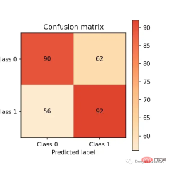
The confusion matrix summarizes the performance of the model in four regions:
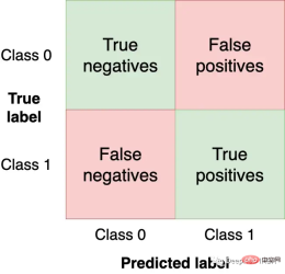
We want to have the top left and Get as many observations (from the test set) in the lower right quadrant as these are the correct observations for our model to get. The other quadrants are model errors.
Changing the model's threshold will change the values in the confusion matrix. In the previous example, using clf.predict, a binary response was returned (i.e. using 0.5 as the threshold); but we can use the clf.predict_proba function to get the raw probability and use a custom threshold:
y_score = clf.predict_proba(X_test)
We can Make our classifier more aggressive by setting a lower threshold (i.e. label more posts as harmful) and create a new confusion matrix:
cm_dot_four = ConfusionMatrix(y_score[:, 1] >= 0.4, y_pred)
The sklearn-evaluation library makes this easy Comparing the two matrices:
cm_dot_five + cm_dot_four
The upper part of the triangle comes from the threshold of 0.5, and the lower part comes from the threshold of 0.4:
- Both models predict 0 for the same number of observations (this is a coincidence). 0.5 threshold: (90 56 = 146). 0.4 threshold: (78 68 = 146)
- Lowering the threshold will result in more false negatives (from 56 cases to 68 cases)
- Lowering the threshold will greatly increase the number of true positives (from 92 cases) Added 154 cases)
Small threshold changes greatly affect the confusion matrix. We only analyzed two thresholds. Then if we can analyze the model performance across all values, we can better understand the threshold dynamics. But before that can happen, new metrics for model evaluation need to be defined.
So far, we have used absolute numbers to evaluate our models. To facilitate comparison and evaluation, we will now define two normalized metrics (their values are between 0.0 and 1.0).
Precision is the proportion of observed events that are labeled (for example, posts that our model considers harmful, they are harmful). Recall is the proportion of actual events retrieved by our model (i.e., out of all harmful posts, which proportion of them we were able to detect).
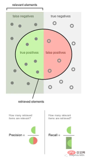
The above picture is from Wikipedia, which can well illustrate how these two indicators are calculated. Precision and recall are both proportional, so they are both 0 than 1 ratio.
Run the experiment
We will obtain precision, recall, and other statistics based on several thresholds to better understand how the thresholds affect them. We will also repeat this experiment multiple times to measure variability.
The commands in this section are all bash commands. They need to be executed in the terminal. If using Jupyter you can use the %%sh magic command.
Here we use Plomber Cloud to run our experiments. Because it allows us to run experiments in parallel and retrieve results quickly.
Created a Notebook that fit a model and calculated statistics for several thresholds, executing the same Notebook 20 times in parallel.
curl -O https://raw.githubusercontent.com/ploomber/posts/master/threshold/fit.ipynb?utm_source=medium&utm_medium=blog&utm_campaign=threshold
Let's execute this notebook (the configuration in the file will tell Plomber Cloud to run it 20 times in parallel):
ploomber cloud nb fit.ipynb
After a few minutes, we will see the 20 experiments complete:
ploomber cloud status @latest --summary

 status count
 -------- -------
 finished 20

 Pipeline finished. Check outputs:
 $ ploomber cloud products
Let’s download the experimental results stored in a .csv file:
ploomber cloud download 'threshold-selection/*.csv' --summary
Visualizing the experimental results
will load the results of all experiments and plot them in one go .
 from glob import glob

 import pandas as pd
 import numpy as np
 paths = glob('threshold-selection/**/*.csv')
 metrics = [pd.read_csv(path) for path in paths]

 for idx, df in enumerate(metrics):
plt.plot(df.threshold, df.precision, color='blue', alpha=0.2,
label='precision' if idx == 0 else None)
plt.plot(df.threshold, df.recall, color='green', alpha=0.2,
label='recall' if idx == 0 else None)
plt.plot(df.threshold, df.f1, color='orange', alpha=0.2,
label='f1' if idx == 0 else None)


 plt.grid()
 plt.legend()
 plt.xlabel('Threshold')
 plt.ylabel('Metric value')

 for handle in plt.legend().legendHandles:
handle.set_alpha(1)

 ax = plt.twinx()

 for idx, df in enumerate(metrics):
ax.plot(df.threshold, df.n_flagged,
label='flagged' if idx == 0 else None,
color='red', alpha=0.2)

 plt.ylabel('Flagged')
 ax.legend(loc=0)
 ax.legend().legendHandles[0].set_alpha(1)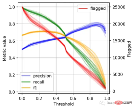
左边的刻度(从0到1)是我们的三个指标:精度、召回率和F1。F1分为精度与查全率的调和平均值,F1分的最佳值为1.0,最差值为0.0;F1对精度和召回率都是相同对待的,所以你可以看到它在两者之间保持平衡。如果你正在处理一个精确度和召回率都很重要的用例,那么最大化F1是一种可以帮助你优化分类器阈值的方法。
这里还包括一条红色曲线(右侧的比例),显示我们的模型标记为有害内容的案例数量。
在这个的内容审核示例中,可能有X个的工作人员来人工审核模型标记的有害帖子,但是他们人数是有限的,因此考虑标记帖子的总数可以帮助我们更好地选择阈值:例如每天只能检查5000个帖子,那么模型找到10,000帖并不会带来任何的提高。如果我人工每天可以处理10000贴,但是模型只标记了100贴,那么显然也是浪费的。
当设置较低的阈值时,有较高的召回率(我们检索了大部分实际上有害的帖子),但精度较低(包含了许多无害的帖子)。如果我们提高阈值,情况就会反转:召回率下降(错过了许多有害的帖子),但精确度很高(大多数标记的帖子都是有害的)。
所以在为我们的二元分类器选择阈值时,我们必须在精度或召回率上妥协,因为没有一个分类器是完美的。我们来讨论一下如何推理选择合适的阈值。
选择最佳阈值
右边的数据会产生噪声(较大的阈值)。需要稍微清理一下,我们将重新创建这个图,我们将绘制2.5%、50%和97.5%的百分位数,而不是绘制所有值。
shape = (df.shape[0], len(metrics))
 precision = np.zeros(shape)
 recall = np.zeros(shape)
 f1 = np.zeros(shape)
 n_flagged = np.zeros(shape)
 for i, df in enumerate(metrics):
precision[:, i] = df.precision.values
recall[:, i] = df.recall.values
f1[:, i] = df.f1.values
n_flagged[:, i] = df.n_flagged.values
 precision_ = np.quantile(precision, q=0.5, axis=1)
 recall_ = np.quantile(recall, q=0.5, axis=1)
 f1_ = np.quantile(f1, q=0.5, axis=1)
 n_flagged_ = np.quantile(n_flagged, q=0.5, axis=1)
 plt.plot(df.threshold, precision_, color='blue', label='precision')
 plt.plot(df.threshold, recall_, color='green', label='recall')
 plt.plot(df.threshold, f1_, color='orange', label='f1')

 plt.fill_between(df.threshold, precision_interval[0],
precision_interval[1], color='blue',
alpha=0.2)

 plt.fill_between(df.threshold, recall_interval[0],
recall_interval[1], color='green',
alpha=0.2)


 plt.fill_between(df.threshold, f1_interval[0],
f1_interval[1], color='orange',
alpha=0.2)
 plt.xlabel('Threshold')
 plt.ylabel('Metric value')
 plt.legend()

 ax = plt.twinx()
 ax.plot(df.threshold, n_flagged_, color='red', label='flagged')
 ax.fill_between(df.threshold, n_flagged_interval[0],
n_flagged_interval[1], color='red',
alpha=0.2)

 ax.legend(loc=3)

 plt.ylabel('Flagged')
 plt.grid()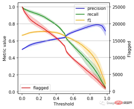
我们可以根据自己的需求选择阈值,例如检索尽可能多的有害帖子(高召回率)是否更重要?还是要有更高的确定性,我们标记的必须是有害的(高精度)?
如果两者都同等重要,那么在这些条件下优化的常用方法就是最大化F-1分数:
idx = np.argmax(f1_)
 prec_lower, prec_upper = precision_interval[0][idx], precision_interval[1][idx]
 rec_lower, rec_upper = recall_interval[0][idx], recall_interval[1][idx]
 threshold = df.threshold[idx]

 print(f'Max F1 score: {f1_[idx]:.2f}')
 print('Metrics when maximizing F1 score:')
 print(f' - Threshold: {threshold:.2f}')
 print(f' - Precision range: ({prec_lower:.2f}, {prec_upper:.2f})')
 print(f' - Recall range: ({rec_lower:.2f}, {rec_upper:.2f})')

 #结果
 Max F1 score: 0.71
 Metrics when maximizing F1 score:
- Threshold: 0.26
- Precision range: (0.58, 0.61)
- Recall range: (0.86, 0.90)
在很多情况下很难决定这个折中,所以加入一些约束条件会有一些帮助。
假设我们有10个人审查有害的帖子,他们可以一起检查5000个。那么让我们看看指标,如果我们修改了阈值,让它标记了大约5000个帖子:
idx = np.argmax(n_flagged_ <= 5000)

 prec_lower, prec_upper = precision_interval[0][idx], precision_interval[1][idx]
 rec_lower, rec_upper = recall_interval[0][idx], recall_interval[1][idx]
 threshold = df.threshold[idx]

 print('Metrics when limiting to a maximum of 5,000 flagged events:')
 print(f' - Threshold: {threshold:.2f}')
 print(f' - Precision range: ({prec_lower:.2f}, {prec_upper:.2f})')
 print(f' - Recall range: ({rec_lower:.2f}, {rec_upper:.2f})')

 # 结果
 Metrics when limiting to a maximum of 5,000 flagged events:
- Threshold: 0.82
- Precision range: (0.77, 0.81)
- Recall range: (0.25, 0.36)
如果需要进行汇报,我们可以在在展示结果时展示一些替代方案:比如在当前约束条件下(5000个帖子)的模型性能,以及如果我们增加团队(比如通过增加一倍的规模),我们可以做得更好。
总结
二元分类器的最佳阈值是针对业务结果进行优化并考虑到流程限制的阈值。通过本文中描述的过程,你可以更好地为用例决定最佳阈值。
另外,Ploomber Cloud!提供一些免费的算力!如果你需要一些免费的服务可以试试它。
The above is the detailed content of Setting the best threshold for machine learning models: Is 0.5 the best threshold for binary classification?. For more information, please follow other related articles on the PHP Chinese website!
 AI Game Development Enters Its Agentic Era With Upheaval's Dreamer PortalMay 02, 2025 am 11:17 AM
Upheaval Games: Revolutionizing Game Development with AI Agents Upheaval, a game development studio comprised of veterans from industry giants like Blizzard and Obsidian, is poised to revolutionize game creation with its innovative AI-powered platfor
 Uber Wants To Be Your Robotaxi Shop, Will Providers Let Them?May 02, 2025 am 11:16 AM
Uber's RoboTaxi Strategy: A Ride-Hail Ecosystem for Autonomous Vehicles At the recent Curbivore conference, Uber's Richard Willder unveiled their strategy to become the ride-hail platform for robotaxi providers. Leveraging their dominant position in
 AI Agents Playing Video Games Will Transform Future RobotsMay 02, 2025 am 11:15 AM
Video games are proving to be invaluable testing grounds for cutting-edge AI research, particularly in the development of autonomous agents and real-world robots, even potentially contributing to the quest for Artificial General Intelligence (AGI). A
 The Startup Industrial Complex, VC 3.0, And James Currier's ManifestoMay 02, 2025 am 11:14 AM
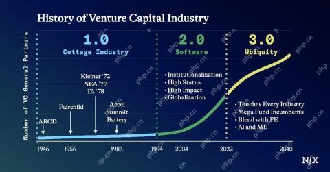
The impact of the evolving venture capital landscape is evident in the media, financial reports, and everyday conversations. However, the specific consequences for investors, startups, and funds are often overlooked. Venture Capital 3.0: A Paradigm
 Adobe Updates Creative Cloud And Firefly At Adobe MAX London 2025May 02, 2025 am 11:13 AM
Adobe MAX London 2025 delivered significant updates to Creative Cloud and Firefly, reflecting a strategic shift towards accessibility and generative AI. This analysis incorporates insights from pre-event briefings with Adobe leadership. (Note: Adob
 Everything Meta Announced At LlamaConMay 02, 2025 am 11:12 AM
Meta's LlamaCon announcements showcase a comprehensive AI strategy designed to compete directly with closed AI systems like OpenAI's, while simultaneously creating new revenue streams for its open-source models. This multifaceted approach targets bo
 The Brewing Controversy Over The Proposition That AI Is Nothing More Than Just Normal TechnologyMay 02, 2025 am 11:10 AM
There are serious differences in the field of artificial intelligence on this conclusion. Some insist that it is time to expose the "emperor's new clothes", while others strongly oppose the idea that artificial intelligence is just ordinary technology. Let's discuss it. An analysis of this innovative AI breakthrough is part of my ongoing Forbes column that covers the latest advancements in the field of AI, including identifying and explaining a variety of influential AI complexities (click here to view the link). Artificial intelligence as a common technology First, some basic knowledge is needed to lay the foundation for this important discussion. There is currently a large amount of research dedicated to further developing artificial intelligence. The overall goal is to achieve artificial general intelligence (AGI) and even possible artificial super intelligence (AS)
 Model Citizens, Why AI Value Is The Next Business YardstickMay 02, 2025 am 11:09 AM
The effectiveness of a company's AI model is now a key performance indicator. Since the AI boom, generative AI has been used for everything from composing birthday invitations to writing software code. This has led to a proliferation of language mod


Hot AI Tools

Undresser.AI Undress
AI-powered app for creating realistic nude photos

AI Clothes Remover
Online AI tool for removing clothes from photos.

Undress AI Tool
Undress images for free

Clothoff.io
AI clothes remover

Video Face Swap
Swap faces in any video effortlessly with our completely free AI face swap tool!

Hot Article

Hot Tools

Dreamweaver Mac version
Visual web development tools

WebStorm Mac version
Useful JavaScript development tools

MinGW - Minimalist GNU for Windows
This project is in the process of being migrated to osdn.net/projects/mingw, you can continue to follow us there. MinGW: A native Windows port of the GNU Compiler Collection (GCC), freely distributable import libraries and header files for building native Windows applications; includes extensions to the MSVC runtime to support C99 functionality. All MinGW software can run on 64-bit Windows platforms.

EditPlus Chinese cracked version
Small size, syntax highlighting, does not support code prompt function

SAP NetWeaver Server Adapter for Eclipse
Integrate Eclipse with SAP NetWeaver application server.


