 Technology peripherals
 AI
AI An article discussing the issues and challenges in autonomous driving decision planning
In the positioning, perception, prediction, decision planning and control modules of autonomous driving, the perception module is like human eyes and ears, responsible for sensing the external environment; the control module is like human hands and feet. It is responsible for the final acceleration, deceleration, steering and other operations; the decision-making planning module is like the human brain, making behavioral decisions and trajectory generation based on the received perception and other information.
Welcome to follow the "Smart Driving Frontier" WeChat video account. Just like the human brain is divided into the left brain and the right brain, the decision-making planning module can be further divided into the behavioral decision-making layer (Behavioral Layer) and the motion planning layer. (Motion Planning).
After receiving the global path, the behavioral decision-making layer combines the sensory information to make specific behavioral decisions; the motion planning layer plans to generate a trajectory that satisfies specific constraints based on the specific behavioral decisions. This trajectory is as Inputs from the control module determine the vehicle's final travel path.
As the level of autonomous driving continues to improve, the importance of the decision-making and planning layer as the brain of autonomous driving has also increased. But compared with the human brain, the brain of autonomous driving still has a long way to catch up. This article will detail the problems and challenges of Motion Planning in path planning through ten thousand words.
01 Commonly used algorithms for Motion Planning
The Motion Planning algorithm was developed from the field of robotics, and has gradually developed various algorithms suitable for the field of autonomous driving. The paper [1] provides an overview of the trajectory generation method of Motion Planning. The introduced method is shown in the figure below.
Algorithms based on sampling search: Dijkstra, RRT, A*, hybridA* and Lattice, etc.;
Algorithms based on curve interpolation: RS curve, Dubins curve, polynomial curve, Bezier curve and spline curves, etc.;
Optimization-based algorithms: Apollo’s piecewise-jerk, etc.;

The above algorithms are generally used in combination with each other of. For example, polynomial curves need to sample terminal states, Bezier curves need to sample control points, and hybird A* uses RS curves or Dubins curves, etc.
The paper [1] summarizes the advantages and disadvantages of various trajectory generation algorithms, as shown in the figure below. It can be seen that no algorithm is perfect, and an appropriate algorithm needs to be selected based on specific scenarios and working conditions. Currently, polynomial curve interpolation (high-speed scenarios) and optimization algorithms are widely used in the industry.

02 Motion Planning issues and challenges
The Motion Planning algorithm introduced above can basically solve most of the trajectory generation problems in autonomous driving scenarios. Trajectory generation Algorithms are no longer the main bottleneck. However, there are still many challenges that need to be overcome in the field of Motion Planning, mainly including the following aspects:
Optimality problem;
Cognitive reasoning problem;
Uncertainty/Probability;
Single-Agent;
Multiple-Agent;
Engineering issues.
2.1 Optimality problem
Global optimization is an NP-hard problem [3]. For real-time performance, most of the industry adopts horizontal and vertical decoupling planning methods. However, doing so will sacrifice optimality, and good vehicle behavior cannot be obtained under some working conditions, such as overtaking [2], oncoming vehicles, centripetal acceleration constraint processing, and horizontal planning that requires consideration of longitudinal planning capabilities.
For example, when there is a decelerating vehicle in front of the Autonomous Driving Car (ADC), the horizontal and vertical decoupling method generally only overtakes when the speed of the vehicle in front reduces to a certain value. . The behavior of ADC is to first slow down or even stop, and then drive around obstacles. This is obviously not the optimal driving strategy.
If a spatio-temporal integrated planning method is adopted, deceleration or parking behaviors can be avoided. The left picture in the figure below is an example of the decoupling method. When there is a decelerating and parking vehicle ahead, the ADC will decelerate. The picture on the right is an example of spatio-temporal planning. ADC will overtake when the vehicle in front slows down.

2.2 Cognitive reasoning problem
2.2.1 Map topology reasoning
Take Apollo as an example, PNC The Map module extracts data from the HD Map module to form a reference line, and queries road elements through the API interface of the HD Map module. However, the Motion Planning module ignores some road topological relationships, such as incoming and outgoing intersections, and these special road topologies will affect vehicle behavior.
In addition, if there is no HD Map module and relies solely on visual lane lines, abnormal lane line perception will occur at this time. The road topology problem is particularly prominent in the incoming and outgoing roads and intersection roads.
2.2.2 Unified modeling of obstacles
Participants in the traffic scene include vehicles, motorcycles, bicycles, pedestrians, cones, etc. Broadly speaking, it also includes static map elements such as crosswalks, traffic lights, and road speed limits. Motion Planning needs to make different decisions for different elements. Unified modeling of obstacles can simplify the problem and improve computational efficiency.

2.2.3 Scenario Cognitive Reasoning
Due to the complexity of the real environment, it is difficult for one decision-making strategy or planning method to handle different working conditions. Therefore, classifying the driving environment and choosing different strategies in different scenarios can improve the performance of Motion Planning. So how to carry out scene classification and scene recognition, and what are the differences between Motion Planning in different scenes? These problems all need to be solved. The scene classification in Aopllo is LANE_FOLLOW, SIDE_PASS, STOP_SIGN_UNPROTECTED, etc. There are two methods of scene recognition, one is through rules and the other is through machine learning. Different scenarios have different stages, and tasks are executed in sequence in the stages. Even the same task may have different parameter configurations in different scenarios. Based on the characteristics of urban scenes with many intersections, congestion and lane changes, Haimou divides driving scenes into ten categories, which is obviously different from the scenario classification in Apollo. However, Haimou's scene recognition method cannot And know. Hao Mo also proposed the concept of driving environment entropy to describe the congestion state of the driving environment. 2.3 Uncertainty2.3.1 Positioning Uncertainty
In most Motion Planning, the positioning is considered to be accurate enough. However, in actual scenes, positioning is often inaccurate due to problems such as occlusion and multipath interference. As shown in the lower left figure in the paper [6], the positioning error causes errors in the road boundary queried from the HD Map module, so that the planning and vehicle driving trajectories are on the road boundary. PictureThe paper assumes that positioning uncertainty is a Gaussian distribution, and the positioning module can calculate the expectation and variance of the probability distribution. The paper converts the vehicle coordinate system to the UTM coordinate system. According to the high-speed distribution of positioning and the coordinate transformation formula, the uncertainty of the vehicle's surrounding environment under the influence of positioning can be calculated, as shown in the figure on the right above, where the darker the color. The greater the uncertainty, the uncertainty calculation formula is mainly obtained by the following formula. It can be found that the farther away from the ADC, the higher the uncertainty. As the vehicle moves forward, its uncertainty will be updated. The path planning method uses the Lattice (quintic polynomial curve) method, and two items are added during cost calculation. One is a hard constraint: the maximum uncertainty of a point on the planning path cannot be greater than a certain threshold; the second is to add the weight sum of uncertainties in the cost function.
2.3.2 Perception uncertainty
Due to sensor noise, vehicle vibration, driving environment and imperfect algorithms, perception The results obtained are uncertain or even wrong. Perceived uncertainty can cause insecurity in Motion Planning results. A simple processing method is to add a buffer, but a rough processing method will reduce the feasible range of Motion Planning and may result in an overly aggressive or overly conservative driving strategy. The paper [7] takes the parking application equipped with Around View Monitoring (AVM) as an example. Due to the perception error, the path planning will cause parking at the actual overtaking position, and a collision may occur, as shown in the left figure below. The paper models the perceived uncertainty as a Gaussian distribution. The farther the perceived effect is from the ADC, the higher the uncertainty, as shown in the right figure below.
Parking space sampling: Sampling the two closest corner points to the ADC, treating the sampling points as normally distributed, and calculating the parking center of the ADC rear axle based on the sampling corner points and the length of the set parking space. point;
Path candidate generation: Use ocp theory to perform path planning for each sampling point, in which the time domain problem is converted into the Ferent coordinate system, and SQP is used to solve the nonlinear problem;
Optimal Path Selection: Use utility theory to select the optimal path. Utility function is: EU(s) = P(s) x Uideal(s) (1-P(s)) x Ureal(s), where P(s) is the probability of the path corresponding to the sampling point, and Uideal is the path to the target. The deviation utility function value of the point (sensingly detected at the current moment, not obtained by sampling), Ureal is the utility function value on the path to the current position of the ADC.

2.3.3 Prediction Uncertainty
Prediction is an important part of realizing high-level autonomous driving above L4. However, as of now, forecasting remains a very difficult problem for the entire industry. Therefore, the accuracy of prediction is very poor, and it is very important to do motion planning under the uncertainty of prediction results.
The paper [8] proposes a planning architecture based on Gaussian distribution to deal with the problem of unsafe planning trajectories caused by uncertainty in prediction and control.
Candidate trajectory generation: generated through multi-stage horizontal and vertical sampling. It can be understood as the Aopllo Lattice method.
Predicted trajectory generation: When predicting (planning) the trajectory of a certain vehicle, it is considered that other vehicles are traveling at a constant speed and their states are determined. Then, by calculating the cost of the candidate trajectory, we get optimal predicted trajectory. The probability distribution of the predicted trajectory is then calculated through Kalman filtering, assuming that it follows a normal distribution.
ADC trajectory generation: At this time, the uncertainty of the predictions of other traffic participants needs to be considered. For each candidate trajectory, the control error is calculated through the LQR algorithm, and then the probability distribution of the trajectory is calculated through Kalman filtering. When cos calculation is performed for trajectory evaluation, collision detection is based on the probability distribution of the predicted and ADC planning trajectories, that is Collisions cannot occur within any probability distribution.
The author believes that this method is equivalent to adding an adaptive buffer to the box, while a conventional fixed-size buffer will lead to conservative or aggressive driving behavior.

Paper [9] The paper proposes a fail-safe mechanism that can be embedded in the existing Motion Planning framework, which is divided into three parts:
Set- based prediction: Based on the developed driving strategies and vehicle kinematics models of traffic participants, the original single predicted trajectory of traffic participants is changed to multiple predicted trajectories;
Fail-safe trajectory: Based on the predicted As a result, the first trajectory point with collision risk in the original planning trajectory is calculated, and then the trajectory is generated based on the optimization theory;
Online verification: Project the ADC on the trajectory generated in the second step to determine whether it is And the first step is to predict whether there is a collision in the vehicle trajectory.
I feel that this method is a re-doing of Motion Planning. Since the paper does not describe whether the fail-safe trajectory considers the decision results, it may cause the safe trajectory not to satisfy the decision results, and this paper is only a simulation, and Has no practical application.

2.3.4 Partially Observable Environments
Due to the limited sensing range of the sensor itself and the uncertainty of the sensing results, in It will be further amplified in bad lighting or bad weather. In urban working conditions, the occlusion of buildings will cause incomplete perception, as shown in the figure below. In addition, large vehicles can also cause perceptual occlusion problems, and most Motion Planning is processed with complete perception, so the planning results are very unsafe.

The paper [10] proposes a motion planning that handles incomplete perception of safety, so that the planned trajectory can be safe under the maximum braking capacity of the vehicle in the most dangerous situations. Park your car without crashing. It is divided into two situations: one is when driving on a straight road, considering the uncertainty of perception and the range of perception distance, and the second is when driving at an urban intersection, where incomplete perception is considered. And it is easy to embed into other Motion Planning architectures. The author conducted simulation verification in the trajectory planning based on the optimization method previously proposed (Figure (b) in the review).
The author designed several assumptions for his theory:
The longitudinal position and velocity information of positioning follows Gaussian distribution;
The effective range of perception is known, and the perception The result follows Gaussian distribution;
The map information contains the location of the building and is a convex polygon;
Use Intelligent Driver Model (IDM) for vehicle acceleration prediction.
Since the paper deals with two situations: straight roads and intersections, scene recognition is required. The paper uses a rule-based approach for scene recognition.

The upper left picture: the red dotted line is the time when the observed environment is sensed, and the black dotted line is the time for Motion Planning. It can be seen that the sensing information used by Motion Planning is before the tp time of. In addition, because Motion Planning must ensure continuity, the planned trajectory within the Motion Planning calculation cycle tpin must be consistent. More importantly, due to the delay of the actuator, the safety of the trajectory must be ensured within the tsafe time. In the paper, tsafe= 2tpin;
Top and middle picture: Driving on a straight road is divided into two situations: there are no vehicles within the sensing range or there are vehicles within the sensing range: First, there are no vehicles within the sensing range, assuming there are vehicles outside the driving sensing range A stationary vehicle is set as a virtual stationary obstacle. Through its Gaussian distribution characteristics, it can be calculated to satisfy the longitudinal displacement and speed constraints of braking with the maximum braking capacity within the tsafe moment; secondly, if there is a vehicle within the sensing range, consider that the sensing is not possible. The most dangerous situation under deterministic conditions, that is, the vehicle in front is braking with the maximum braking capacity. Through its Gaussian distribution characteristics, it can be calculated to satisfy the longitudinal displacement and speed constraints of braking with the maximum braking capacity within the tsafe time;
Above right picture: Driving at an intersection, according to the IDM model, it is calculated whether the ADC needs to give way or has the right of way and needs to clearly indicate its intention to pass first. Finally converted to two types of constraints for straight driving.
2.4 Single Agent
Single Agent considers it a single agent problem, that is, the ADC will make decisions about the surrounding environment without considering the impact of the ADC's behavioral decisions on other traffic participants. Obviously this This assumption is incorrect, but it simplifies the Motion Planning problem.
Behavioral decision-making is another important aspect that affects the development of autonomous driving. As the level of autonomous driving increases, the importance of behavioral decision-making becomes higher. The difficulty in behavioral decision-making is how to embody the intelligence of autonomous vehicles and how to enable autonomous vehicles to handle high-dimensional, multi-constraint complex scenarios like human drivers, or even perform better than human drivers.
Most current methods are rule-based methods with limited capabilities. In terms of behavioral decision-making based on the rule method, in off-ramp conditions, a distance threshold from the ramp entrance is generally designed. When the distance from the ADC to the ramp is within the threshold, the lane change to the rightmost lane begins.
Assuming that this threshold is 2km, if the ADC is driving in the middle lane at 2.1m of the ramp intersection, and there is a car in front at a low speed, the rule-based behavioral decision-making will generally choose to change to the left lane. (the left lane has a high speed limit, and overtaking must follow the left lane. It can be seen from Xiaopeng NGP and others that the left lane has priority). However, the distance threshold to the ramp entrance after changing lanes is less than 2km. At this time, it is necessary to change lanes to the rightmost lane, and it is necessary to perform two consecutive lane changes, which will appear not smart enough.
Another example is driving in the rightmost lane 500m before the ramp. If the road ahead cannot be driven due to construction or an accident, the driver can only take over. It can be seen that due to the complexity of real-life working conditions, it is difficult to achieve a good driving experience with a rule-based behavioral decision-making method.
Hong Kong University of Science and Technology's behavioral decision-making work on OPMDP [11] has a certain improvement in performance compared to the rule-based method. It prunes the behavior of ADC and other traffic participants, reducing the OPMDP time consuming. However, it takes into account that other traffic participants will avoid the ADC's behavior, etc. It can be seen that it is a Multiple Agent problem to deal with.
2.5 Multiple Agent
In the above-mentioned Single Agent, it is believed that traffic participants will not make corresponding decisions on the behavior of the ADC. But in reality, when the ADC makes After the decision is made, its behavior will affect the behavior of other traffic participants, reducing the credibility of the original prediction results. In particular, some simple rule-based predictions do not depend on the Motion Planning results, or use the previous frame of Motion Planning. The result (Apollo).
For example, in the left picture below, when ADC L is traveling along trajectory 1, A2 may slow down to avoid it. As ADC L travels along trajectory 2, A2 may accelerate through the intersection. But when ADC L is driving along trajectory 2, it is predicted that A2 may accelerate through the intersection, but A2 may misunderstand ADC L's intention and slow down, causing the two vehicles to lock up. Therefore, how ADC understands the intentions of other traffic participants and how other traffic vehicles understand the intentions of ADC is crucial [12].

2.6 Engineering issues
We also face some engineering issues in Motion Planning, mainly including the following aspects.
Real-time: The optimality problem mentioned in the first question. If it is to be solved, due to the complexity of search calculations in three-dimensional space, its real-time performance can be guaranteed. This also limits the application of joint spatio-temporal planning. A reason. In addition, large-scale constraints and nonlinearity in the optimization algorithm also face real-time challenges.
Completeness: Algorithms such as interpolation and Lattice are probabilistically complete. Especially in complex multi-obstacle environments, it is difficult to obtain a collision-free trajectory with limited sampling. The optimization method cannot achieve completeness due to numerical solution, and the commonly used osqp solver may even give an incorrect solution.
Difficult to quantify: Most of the evaluation indicators in Motion Planning are subjective, such as comfort and passability, etc., which are difficult to quantitatively evaluate. Different engineers adjust the parameters to get different body sensations, which are also different from the subjective feelings of passengers. Therefore, machine learning methods are proposed to learn parameters or lane changing strategies in Motion Planning.
03 Industry Solutions
In response to the above problems and challenges, companies in the industry are also actively exploring and proposing some solutions, one or two of which are listed below.
Qingzhou Zhihang uses space-time joint planning to solve the optimality problem, improve planning performance, and develops a self-developed nonlinear planner for efficient solution [2].
In the new generation framework of TuSimple, the perception module provides uncertainty or probability information while providing information such as obstacle location and speed to ensure that decision-making planning can make safe and comfortable decisions in advance [13 ].
Tesla uses Planner for other vehicles used by traffic participants. However, when interacting with other vehicles, planning should not be just for the ADC, but should be planned jointly for all traffic participants and optimized for the traffic flow of the overall scene. To do this, the autopilot planner is run for each participating object in the scene. In addition, for parking scenarios, the A search algorithm and neural network combination strategy are used, which greatly reduces the node exploration of the A algorithm [15].
Xpeng and Tesla have optimized the problem of missing lane lines and changes in road topology [14].
Waymo proposed ChauffeurNet to improve decision-making performance [16], and Apollo proposed its own reinforcement learning architecture based on ChauffeurNet [17].
The above is the detailed content of An article discussing the issues and challenges in autonomous driving decision planning. For more information, please follow other related articles on the PHP Chinese website!
 在 CARLA自动驾驶模拟器中添加真实智体行为Apr 08, 2023 pm 02:11 PM
arXiv论文“Insertion of real agents behaviors in CARLA autonomous driving simulator“,22年6月,西班牙。由于需要快速prototyping和广泛测试,仿真在自动驾驶中的作用变得越来越重要。基于物理的模拟具有多种优势和益处,成本合理,同时消除了prototyping、驾驶员和弱势道路使用者(VRU)的风险。然而,主要有两个局限性。首先,众所周知的现实差距是指现实和模拟之间的差异,阻碍模拟自主驾驶体验去实现有效的现实世界
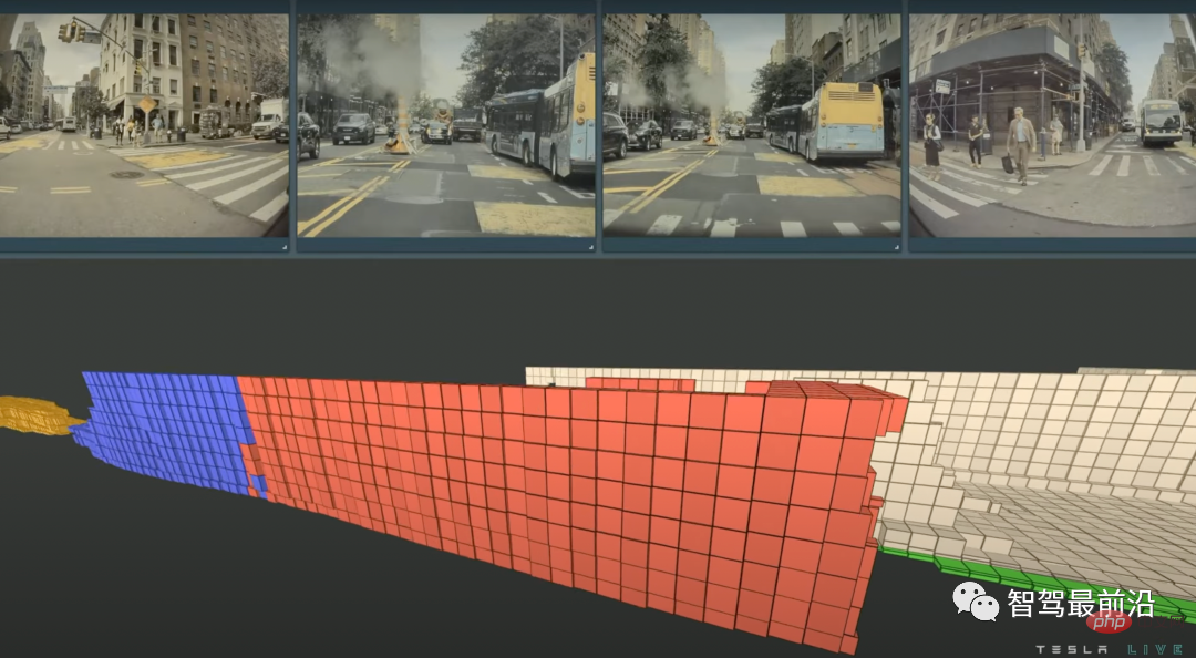 特斯拉自动驾驶算法和模型解读Apr 11, 2023 pm 12:04 PM
特斯拉是一个典型的AI公司,过去一年训练了75000个神经网络,意味着每8分钟就要出一个新的模型,共有281个模型用到了特斯拉的车上。接下来我们分几个方面来解读特斯拉FSD的算法和模型进展。01 感知 Occupancy Network特斯拉今年在感知方面的一个重点技术是Occupancy Network (占据网络)。研究机器人技术的同学肯定对occupancy grid不会陌生,occupancy表示空间中每个3D体素(voxel)是否被占据,可以是0/1二元表示,也可以是[0, 1]之间的
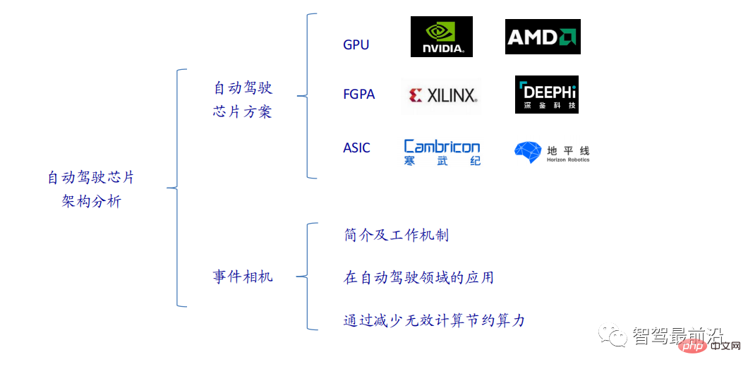 一文通览自动驾驶三大主流芯片架构Apr 12, 2023 pm 12:07 PM
当前主流的AI芯片主要分为三类,GPU、FPGA、ASIC。GPU、FPGA均是前期较为成熟的芯片架构,属于通用型芯片。ASIC属于为AI特定场景定制的芯片。行业内已经确认CPU不适用于AI计算,但是在AI应用领域也是必不可少。 GPU方案GPU与CPU的架构对比CPU遵循的是冯·诺依曼架构,其核心是存储程序/数据、串行顺序执行。因此CPU的架构中需要大量的空间去放置存储单元(Cache)和控制单元(Control),相比之下计算单元(ALU)只占据了很小的一部分,所以CPU在进行大规模并行计算
 自动驾驶汽车激光雷达如何做到与GPS时间同步?Mar 31, 2023 pm 10:40 PM
gPTP定义的五条报文中,Sync和Follow_UP为一组报文,周期发送,主要用来测量时钟偏差。 01 同步方案激光雷达与GPS时间同步主要有三种方案,即PPS+GPRMC、PTP、gPTPPPS+GPRMCGNSS输出两条信息,一条是时间周期为1s的同步脉冲信号PPS,脉冲宽度5ms~100ms;一条是通过标准串口输出GPRMC标准的时间同步报文。同步脉冲前沿时刻与GPRMC报文的发送在同一时刻,误差为ns级别,误差可以忽略。GPRMC是一条包含UTC时间(精确到秒),经纬度定位数据的标准格
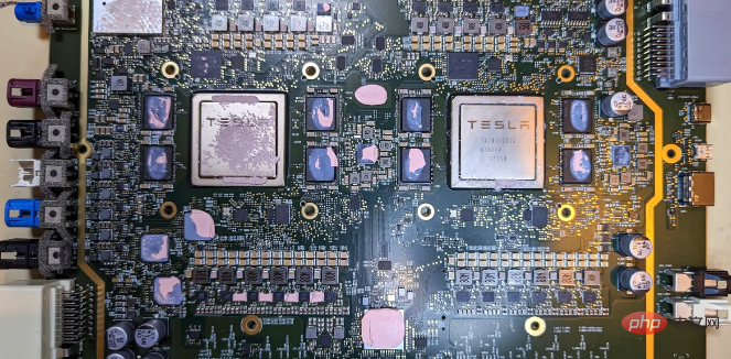 特斯拉自动驾驶硬件 4.0 实物拆解:增加雷达,提供更多摄像头Apr 08, 2023 pm 12:11 PM
2 月 16 日消息,特斯拉的新自动驾驶计算机,即硬件 4.0(HW4)已经泄露,该公司似乎已经在制造一些带有新系统的汽车。我们已经知道,特斯拉准备升级其自动驾驶硬件已有一段时间了。特斯拉此前向联邦通信委员会申请在其车辆上增加一个新的雷达,并称计划在 1 月份开始销售,新的雷达将意味着特斯拉计划更新其 Autopilot 和 FSD 的传感器套件。硬件变化对特斯拉车主来说是一种压力,因为该汽车制造商一直承诺,其自 2016 年以来制造的所有车辆都具备通过软件更新实现自动驾驶所需的所有硬件。事实证
 端到端自动驾驶中轨迹引导的控制预测:一个简单有力的基线方法TCPApr 10, 2023 am 09:01 AM
arXiv论文“Trajectory-guided Control Prediction for End-to-end Autonomous Driving: A Simple yet Strong Baseline“, 2022年6月,上海AI实验室和上海交大。当前的端到端自主驾驶方法要么基于规划轨迹运行控制器,要么直接执行控制预测,这跨越了两个研究领域。鉴于二者之间潜在的互利,本文主动探索两个的结合,称为TCP (Trajectory-guided Control Prediction)。具
 一文聊聊自动驾驶中交通标志识别系统Apr 12, 2023 pm 12:34 PM
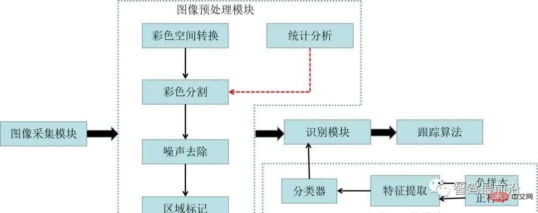
什么是交通标志识别系统?汽车安全系统的交通标志识别系统,英文翻译为:Traffic Sign Recognition,简称TSR,是利用前置摄像头结合模式,可以识别常见的交通标志 《 限速、停车、掉头等)。这一功能会提醒驾驶员注意前面的交通标志,以便驾驶员遵守这些标志。TSR 功能降低了驾驶员不遵守停车标志等交通法规的可能,避免了违法左转或者无意的其他交通违法行为,从而提高了安全性。这些系统需要灵活的软件平台来增强探测算法,根据不同地区的交通标志来进行调整。交通标志识别原理交通标志识别又称为TS
 一文聊聊SLAM技术在自动驾驶的应用Apr 09, 2023 pm 01:11 PM
定位在自动驾驶中占据着不可替代的地位,而且未来有着可期的发展。目前自动驾驶中的定位都是依赖RTK配合高精地图,这给自动驾驶的落地增加了不少成本与难度。试想一下人类开车,并非需要知道自己的全局高精定位及周围的详细环境,有一条全局导航路径并配合车辆在该路径上的位置,也就足够了,而这里牵涉到的,便是SLAM领域的关键技术。什么是SLAMSLAM (Simultaneous Localization and Mapping),也称为CML (Concurrent Mapping and Localiza


Hot AI Tools

Undresser.AI Undress
AI-powered app for creating realistic nude photos

AI Clothes Remover
Online AI tool for removing clothes from photos.

Undress AI Tool
Undress images for free

Clothoff.io
AI clothes remover

AI Hentai Generator
Generate AI Hentai for free.

Hot Article

Hot Tools

SublimeText3 Mac version
God-level code editing software (SublimeText3)

MinGW - Minimalist GNU for Windows
This project is in the process of being migrated to osdn.net/projects/mingw, you can continue to follow us there. MinGW: A native Windows port of the GNU Compiler Collection (GCC), freely distributable import libraries and header files for building native Windows applications; includes extensions to the MSVC runtime to support C99 functionality. All MinGW software can run on 64-bit Windows platforms.

Atom editor mac version download
The most popular open source editor

Dreamweaver CS6
Visual web development tools

VSCode Windows 64-bit Download
A free and powerful IDE editor launched by Microsoft


