

 Technology peripheralsAIIt's easy to build and train your first neural network with TensorFlow and Keras
AI technology is developing rapidly. Using various advanced AI models, chat robots, humanoid robots, self-driving cars, etc. can be created. AI has become the fastest growing technology, and object detection and object classification are recent trends.
This article will introduce the complete steps of building and training an image classification model from scratch using a convolutional neural network. This article will use the public Cifar-10 data set to train this model. This dataset is unique because it contains images of everyday objects like cars, airplanes, dogs, cats, etc. By training a neural network on these objects, this article will develop an intelligent system to classify these things in the real world. It contains more than 60,000 32x32 images of 10 different types of objects. By the end of this tutorial, you will have a model that can identify objects based on their visual characteristics.
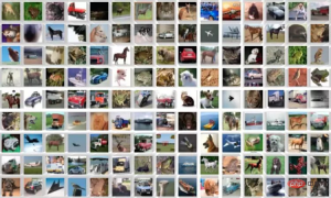
Figure 1 Dataset sample image|Picture from datasets.activeloop
This article will tell everything from the beginning, so if you haven’t learned neural networks yet The actual implementation is completely fine.
The following is the complete workflow of this tutorial:
- Import the necessary libraries
- Load data
- Preprocessing of data
- Build the model
- Evaluate the performance of the model
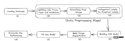
Figure 2 Complete process
Import the necessary libraries
You must first install some modules to start this project. This article will use Google Colab because it provides free GPU training.
The following are the commands to install the required libraries:
<code>$ pip install tensorflow, numpy, keras, sklearn, matplotlib</code>
Import the libraries into the Python file.
<code>from numpy import *from pandas import *import matplotlib.pyplot as plotter# 将数据分成训练集和测试集。from sklearn.model_selection import train_test_split# 用来评估我们的训练模型的库。from sklearn.metrics import classification_report, confusion_matriximport keras# 加载我们的数据集。from keras.datasets import cifar10# 用于数据增量。from keras.preprocessing.image import ImageDataGenerator# 下面是一些用于训练卷积Nueral网络的层。from keras.models import Sequentialfrom keras.layers import Dense, Dropout, Activationfrom keras.layers import Conv2D, MaxPooling2D, GlobalMaxPooling2D, Flatten</code>
- Numpy: It is used for efficient array calculations on large data sets containing images.
- Tensorflow: It is an open source machine learning library developed by Google. It provides many functions to build large and scalable models.
- Keras: Another high-level neural network API running on top of TensorFlow.
- Matplotlib: This Python library can create charts and provide better data visualization.
- Sklearn: It provides functions to perform data preprocessing and feature extraction tasks on data sets. It contains built-in functions to find model evaluation metrics such as accuracy, precision, false positives, false negatives, etc.
Now, enter the data loading step.
Loading data
This section will load the data set and perform the training-test data split.
Loading and splitting data:
<code># 类的数量nc = 10(training_data, training_label), (testing_data, testing_label) = cifar10.load_data()((training_data),(validation_data),(training_label),(validation_label),) = train_test_split(training_data, training_label, test_size=0.2, random_state=42)training_data = training_data.astype("float32")testing_data = testing_data.astype("float32")validation_data = validation_data.astype("float32")</code>
The cifar10 dataset is loaded directly from the Keras dataset library. And these data are also divided into training data and test data. Training data is used to train the model so that it can recognize patterns in it. While the test data is invisible to the model, it is used to check its performance, i.e. how many data points are correctly predicted relative to the total number of data points.
training_label contains the label corresponding to the image in training_data.
Then use the built-in sklearn's train_test_split function to split the training data into validation data again. Validation data were used to select and tune the final model. Finally, all training, testing and validation data are converted to 32-bit floating point numbers.
Now, the loading of the data set has been completed. In the next section, this article performs some preprocessing steps on it.
Data preprocessing
Data preprocessing is the first and most critical step in developing a machine learning model. Follow this article to find out how to do this.
<code># 归一化training_data /= 255testing_data /= 255validation_data /= 255# 热编码training_label = keras.utils.to_categorical(training_label, nc)testing_label = keras.utils.to_categorical(testing_label, nc)validation_label = keras.utils.to_categorical(validation_label, nc)# 输出数据集print("Training: ", training_data.shape, len(training_label))print("Validation: ", validation_data.shape, len(validation_label))print("Testing: ", testing_data.shape, len(testing_label))</code>
Output:
<code>Training:(40000, 32, 32, 3) 40000Validation:(10000, 32, 32, 3) 10000Testing:(10000, 32, 32, 3) 10000</code>
This dataset contains images of 10 categories, each image is 32x32 pixels in size. Each pixel has a value from 0-255, and we need to normalize it between 0-1 to simplify the calculation process. After that, we will convert the categorical labels into one-hot encoded labels. This is done to convert categorical data into numerical data so that we can apply machine learning algorithms without any problem.
Now, enter the construction of CNN model.
Building CNN model
The CNN model works in three stages. The first stage consists of convolutional layers to extract relevant features from the image. The second stage consists of pooling layers to reduce the size of the image. It also helps reduce overfitting of the model. The third stage consists of dense layers that convert the 2D image into a 1D array. Finally, this array is fed into the fully connected layer to make the final prediction.
The following is the code:
<code>model = Sequential()model.add(Conv2D(32, (3, 3), padding="same", activatinotallow="relu", input_shape=(32, 32, 3)))model.add(Conv2D(32, (3, 3), padding="same", activatinotallow="relu"))model.add(MaxPooling2D((2, 2)))model.add(Dropout(0.25))model.add(Conv2D(64, (3, 3), padding="same", activatinotallow="relu"))model.add(Conv2D(64, (3, 3), padding="same", activatinotallow="relu"))model.add(MaxPooling2D((2, 2)))model.add(Dropout(0.25))model.add(Conv2D(96, (3, 3), padding="same", activatinotallow="relu"))model.add(Conv2D(96, (3, 3), padding="same", activatinotallow="relu"))model.add(MaxPooling2D((2, 2)))model.add(Flatten())model.add(Dropout(0.4))model.add(Dense(256, activatinotallow="relu"))model.add(Dropout(0.4))model.add(Dense(128, activatinotallow="relu"))model.add(Dropout(0.4))model.add(Dense(nc, activatinotallow="softmax"))</code>
This article applies three groups of layers, each group contains two convolutional layers, a maximum pooling layer and a dropout layer. The Conv2D layer receives input_shape as (32, 32, 3), which must be the same size as the image.
Each Conv2D layer also needs an activation function, namely relu. Activation functions are used to increase nonlinearity in the system. More simply, it determines whether a neuron needs to be activated based on a certain threshold. There are many types of activation functions, such as ReLu, Tanh, Sigmoid, Softmax, etc., which use different algorithms to determine the firing of neurons.
之后,添加了平坦层和全连接层,在它们之间还有几个Dropout层。Dropout层随机地拒绝一些神经元对网层的贡献。它里面的参数定义了拒绝的程度。它主要用于避免过度拟合。
下面是一个CNN模型架构的示例图像。
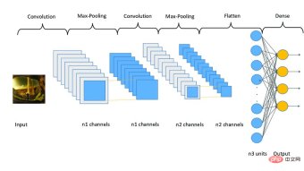
图3 Sampe CNN架构|图片来源:Researchgate
编译模型
现在,本文将编译和准备训练的模型。
<code># 启动Adam优化器opt = keras.optimizers.Adam(lr=0.0001)model.compile(loss="categorical_crossentropy", optimizer=opt, metrics=["accuracy"])# 获得模型的摘要model.summary()</code>
输出:
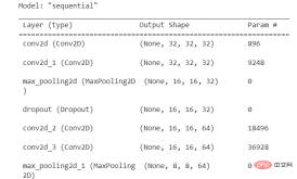
图4 模型摘要
本文使用了学习率为0.0001的Adam优化器。优化器决定了模型的行为如何响应损失函数的输出而变化。学习率是训练期间更新权重的数量或步长。它是一个可配置的超参数,不能太小或太大。
拟合模型
现在,本文将把模型拟合到我们的训练数据,并开始训练过程。但在此之前,本文将使用图像增强技术来增加样本图像的数量。
卷积神经网络中使用的图像增强技术将增加训练图像,而不需要新的图像。它将通过在图像中产生一定量的变化来复制图像。它可以通过将图像旋转到一定程度、添加噪声、水平或垂直翻转等方式来实现。
<code>augmentor = ImageDataGenerator(width_shift_range=0.4,height_shift_range=0.4,horizontal_flip=False,vertical_flip=True,)# 在augmentor中进行拟合augmentor.fit(training_data)# 获得历史数据history = model.fit(augmentor.flow(training_data, training_label, batch_size=32),epochs=100,validation_data=(validation_data, validation_label),)</code>
输出:
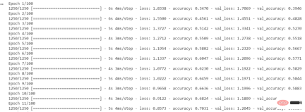
图5 每个时期的准确度和损失
ImageDataGenerator()函数用于创建增强的图像。fit()用于拟合模型。它以训练和验证数据、Batch Size和Epochs的数量作为输入。
Batch Size是在模型更新之前处理的样本数量。一个关键的超参数必须大于等于1且小于等于样本数。通常情况下,32或64被认为是最好的Batch Size。
Epochs的数量代表了所有样本在网络的前向和后向都被单独处理了多少次。100个epochs意味着整个数据集通过模型100次,模型本身运行100次。
我们的模型已经训练完毕,现在我们将评估它在测试集上的表现。
评估模型性能
本节将在测试集上检查模型的准确性和损失。此外,本文还将绘制训练和验证数据的准确率与时间之间和损失与时间之间的关系图。
<code>model.evaluate(testing_data, testing_label)</code>
输出:
<code>313/313 [==============================] - 2s 5ms/step - loss: 0.8554 - accuracy: 0.7545[0.8554493188858032, 0.7545000195503235]</code>
本文的模型达到了75.34%的准确率,损失为0.8554。这个准确率还可以提高,因为这不是一个最先进的模型。本文用这个模型来解释建立模型的过程和流程。CNN模型的准确性取决于许多因素,如层的选择、超参数的选择、使用的数据集的类型等。
现在我们将绘制曲线来检查模型中的过度拟合情况。
<code>def acc_loss_curves(result, epochs):acc = result.history["accuracy"]# 获得损失和准确性loss = result.history["loss"]# 声明损失和准确度的值val_acc = result.history["val_accuracy"]val_loss = result.history["val_loss"]# 绘制图表plotter.figure(figsize=(15, 5))plotter.subplot(121)plotter.plot(range(1, epochs), acc[1:], label="Train_acc")plotter.plot(range(1, epochs), val_acc[1:], label="Val_acc")# 给予绘图的标题plotter.title("Accuracy over " + str(epochs) + " Epochs", size=15)plotter.legend()plotter.grid(True)# 传递值122plotter.subplot(122)# 使用训练损失plotter.plot(range(1, epochs), loss[1:], label="Train_loss")plotter.plot(range(1, epochs), val_loss[1:], label="Val_loss")# 使用 ephocsplotter.title("Loss over " + str(epochs) + " Epochs", size=15)plotter.legend()# 传递真值plotter.grid(True)# 打印图表plotter.show()acc_loss_curves(history, 100)</code>
输出:
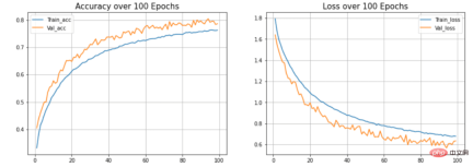
图6 准确度和损失与历时的关系
在本文的模型中,可以看到模型过度拟合测试数据集。(蓝色)线表示训练精度,(橙色)线表示验证精度。训练精度持续提高,但验证误差在20个历时后恶化。
总结
本文展示了构建和训练卷积神经网络的整个过程。最终得到了大约75%的准确率。你可以使用超参数并使用不同的卷积层和池化层来提高准确性。你也可以尝试迁移学习,它使用预先训练好的模型,如ResNet或VGGNet,并在某些情况下可以提供非常好的准确性。
The above is the detailed content of It's easy to build and train your first neural network with TensorFlow and Keras. For more information, please follow other related articles on the PHP Chinese website!

 GNN的基础、前沿和应用Apr 11, 2023 pm 11:40 PM
近年来,图神经网络(GNN)取得了快速、令人难以置信的进展。图神经网络又称为图深度学习、图表征学习(图表示学习)或几何深度学习,是机器学习特别是深度学习领域增长最快的研究课题。本次分享的题目为《GNN的基础、前沿和应用》,主要介绍由吴凌飞、崔鹏、裴健、赵亮几位学者牵头编撰的综合性书籍《图神经网络基础、前沿与应用》中的大致内容。一、图神经网络的介绍1、为什么要研究图?图是一种描述和建模复杂系统的通用语言。图本身并不复杂,它主要由边和结点构成。我们可以用结点表示任何我们想要建模的物体,可以用边表示两
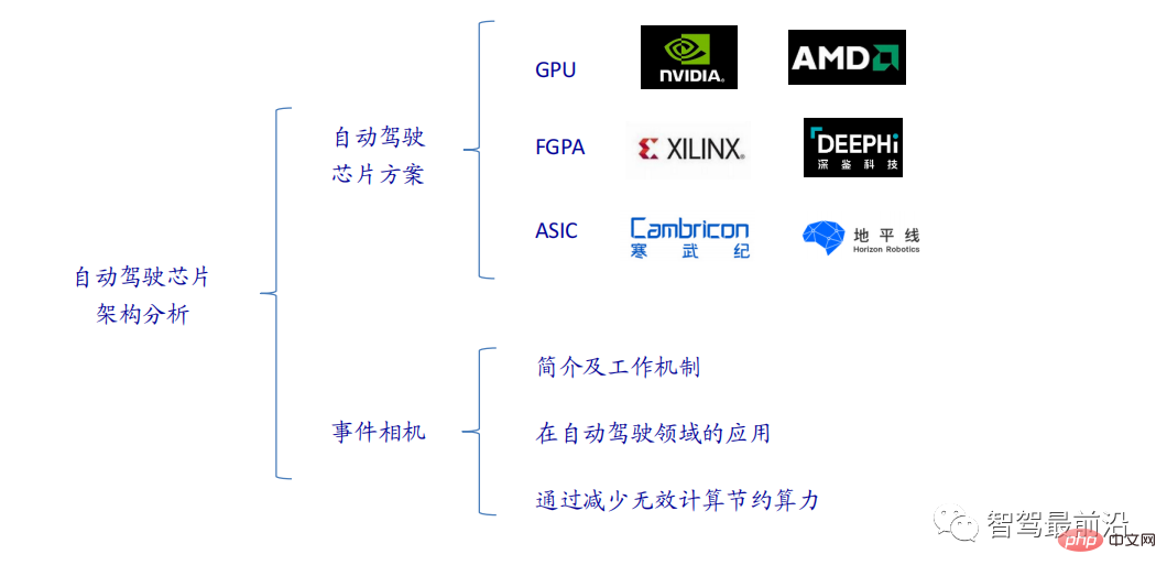 一文通览自动驾驶三大主流芯片架构Apr 12, 2023 pm 12:07 PM
当前主流的AI芯片主要分为三类,GPU、FPGA、ASIC。GPU、FPGA均是前期较为成熟的芯片架构,属于通用型芯片。ASIC属于为AI特定场景定制的芯片。行业内已经确认CPU不适用于AI计算,但是在AI应用领域也是必不可少。 GPU方案GPU与CPU的架构对比CPU遵循的是冯·诺依曼架构,其核心是存储程序/数据、串行顺序执行。因此CPU的架构中需要大量的空间去放置存储单元(Cache)和控制单元(Control),相比之下计算单元(ALU)只占据了很小的一部分,所以CPU在进行大规模并行计算
 "B站UP主成功打造全球首个基于红石的神经网络在社交媒体引起轰动,得到Yann LeCun的点赞赞赏"May 07, 2023 pm 10:58 PM
在我的世界(Minecraft)中,红石是一种非常重要的物品。它是游戏中的一种独特材料,开关、红石火把和红石块等能对导线或物体提供类似电流的能量。红石电路可以为你建造用于控制或激活其他机械的结构,其本身既可以被设计为用于响应玩家的手动激活,也可以反复输出信号或者响应非玩家引发的变化,如生物移动、物品掉落、植物生长、日夜更替等等。因此,在我的世界中,红石能够控制的机械类别极其多,小到简单机械如自动门、光开关和频闪电源,大到占地巨大的电梯、自动农场、小游戏平台甚至游戏内建的计算机。近日,B站UP主@
 扛住强风的无人机?加州理工用12分钟飞行数据教会无人机御风飞行Apr 09, 2023 pm 11:51 PM
当风大到可以把伞吹坏的程度,无人机却稳稳当当,就像这样:御风飞行是空中飞行的一部分,从大的层面来讲,当飞行员驾驶飞机着陆时,风速可能会给他们带来挑战;从小的层面来讲,阵风也会影响无人机的飞行。目前来看,无人机要么在受控条件下飞行,无风;要么由人类使用遥控器操作。无人机被研究者控制在开阔的天空中编队飞行,但这些飞行通常是在理想的条件和环境下进行的。然而,要想让无人机自主执行必要但日常的任务,例如运送包裹,无人机必须能够实时适应风况。为了让无人机在风中飞行时具有更好的机动性,来自加州理工学院的一组工
 对比学习算法在转转的实践Apr 11, 2023 pm 09:25 PM
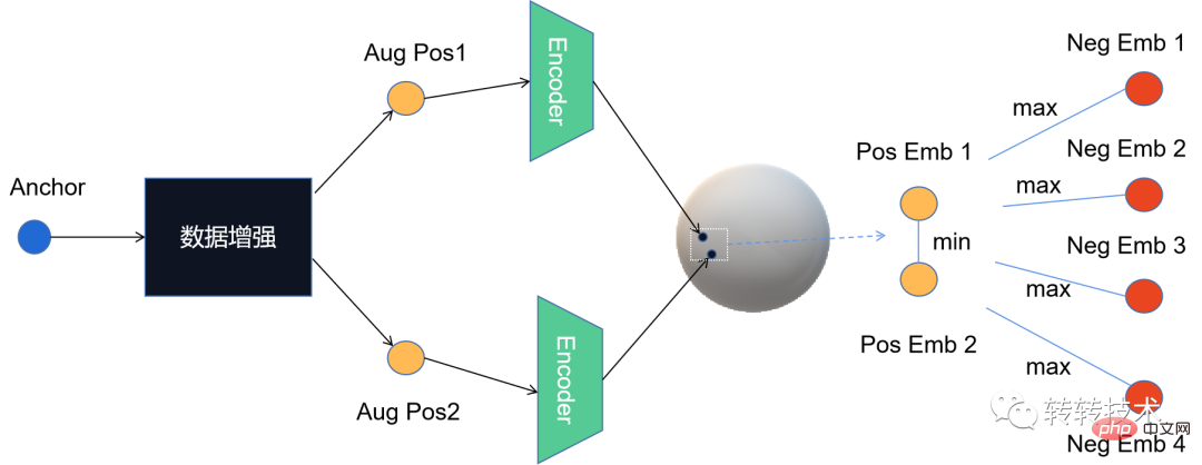
1 什么是对比学习1.1 对比学习的定义1.2 对比学习的原理1.3 经典对比学习算法系列2 对比学习的应用3 对比学习在转转的实践3.1 CL在推荐召回的实践3.2 CL在转转的未来规划1 什么是对比学习1.1 对比学习的定义对比学习(Contrastive Learning, CL)是近年来 AI 领域的热门研究方向,吸引了众多研究学者的关注,其所属的自监督学习方式,更是在 ICLR 2020 被 Bengio 和 LeCun 等大佬点名称为 AI 的未来,后陆续登陆 NIPS, ACL,
 Michael Bronstein从代数拓扑学取经,提出了一种新的图神经网络计算结构!Apr 09, 2023 pm 10:11 PM
本文由Cristian Bodnar 和Fabrizio Frasca 合著,以 C. Bodnar 、F. Frasca 等人发表于2021 ICML《Weisfeiler and Lehman Go Topological: 信息传递简单网络》和2021 NeurIPS 《Weisfeiler and Lehman Go Cellular: CW 网络》论文为参考。本文仅是通过微分几何学和代数拓扑学的视角讨论图神经网络系列的部分内容。从计算机网络到大型强子对撞机中的粒子相互作用,图可以用来模
 微软提出自动化神经网络训练剪枝框架OTO,一站式获得高性能轻量化模型Apr 04, 2023 pm 12:50 PM
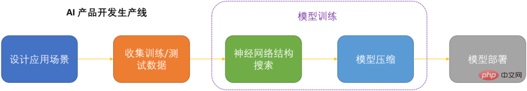
OTO 是业内首个自动化、一站式、用户友好且通用的神经网络训练与结构压缩框架。 在人工智能时代,如何部署和维护神经网络是产品化的关键问题考虑到节省运算成本,同时尽可能小地损失模型性能,压缩神经网络成为了 DNN 产品化的关键之一。DNN 压缩通常来说有三种方式,剪枝,知识蒸馏和量化。剪枝旨在识别并去除冗余结构,给 DNN 瘦身的同时尽可能地保持模型性能,是最为通用且有效的压缩方法。三种方法通常来讲可以相辅相成,共同作用来达到最佳的压缩效果。然而现存的剪枝方法大都只针对特定模型,特定任务,且需要很
 用AI寻找大屠杀后失散的亲人!谷歌工程师研发人脸识别程序,可识别超70万张二战时期老照片Apr 08, 2023 pm 04:21 PM
AI面部识别领域又开辟新业务了?这次,是鉴别二战时期老照片里的人脸图像。近日,来自谷歌的一名软件工程师Daniel Patt 研发了一项名为N2N(Numbers to Names)的 AI人脸识别技术,它可识别二战前欧洲和大屠杀时期的照片,并将他们与现代的人们联系起来。用AI寻找失散多年的亲人2016年,帕特在参观华沙波兰裔犹太人纪念馆时,萌生了一个想法。这一张张陌生的脸庞,会不会与自己存在血缘的联系?他的祖父母/外祖父母中有三位是来自波兰的大屠杀幸存者,他想帮助祖母找到被纳粹杀害的家人的照


Hot AI Tools

Undresser.AI Undress
AI-powered app for creating realistic nude photos

AI Clothes Remover
Online AI tool for removing clothes from photos.

Undress AI Tool
Undress images for free

Clothoff.io
AI clothes remover

AI Hentai Generator
Generate AI Hentai for free.

Hot Article
Hot Tools

Safe Exam Browser
Safe Exam Browser is a secure browser environment for taking online exams securely. This software turns any computer into a secure workstation. It controls access to any utility and prevents students from using unauthorized resources.

SublimeText3 Linux new version
SublimeText3 Linux latest version

VSCode Windows 64-bit Download
A free and powerful IDE editor launched by Microsoft

Atom editor mac version download
The most popular open source editor

SublimeText3 Mac version
God-level code editing software (SublimeText3)

