Sales forecast using LSTM (Python code)

We often encounter scenarios that require prediction, such as predicting brand sales and predicting product sales.

Today I would like to share with you the complete code and detailed explanation of using LSTM for end-to-end time series prediction.

Let’s first understand two topics:

• What is time series analysis?
• What is LSTM?
  

Time series analysis: Time series represents a series of data based on time order. It can be seconds, minutes, hours, days, weeks, months, years. Future data will depend on its previous value.

In real world cases, we have two main types of time series analysis:

• Univariate time series
  
• Multivariate time series
  

For univariate time series data, we will use a single column for forecasting.

#As we can see there is only one column so the upcoming future value will only depend on its previous value.

But in case of multivariate time series data, there will be different types of feature values ​​and the target data will depend on these features.

#As you can see in the picture, there will be multiple columns in the multivariate variable to predict the target value. ("count" in the above figure is the target value)

In the above data, count not only depends on its previous value, but also depends on other features. Therefore, to predict the upcoming count value, we have to consider all columns including the target column to make a prediction for the target value.

One thing must be kept in mind while performing multivariate time series analysis, we need to predict the current target using multiple features, let us understand through an example:

When training, if we use 5 columns [feature1, feature2, feature3, feature4, target] to train the model, we need to provide 4 columns [feature1, feature2, feature3, feature4] for the upcoming prediction day.

LSTM

This article does not intend to discuss LSTM in detail. So I only provide some simple descriptions. If you don’t know much about LSTM, you can refer to our previous articles.

LSTM is basically a recurrent neural network capable of handling long-term dependencies.

Suppose you are watching a movie. So when anything happens in the movie, you already know what happened before and understand that something new is happening because of what happened in the past. RNNs work the same way, they remember past information and use it to process current input. The problem with RNNs is that they cannot remember long-term dependencies due to vanishing gradients. Therefore, lstm was designed to avoid long-term dependency problems.

Now we discuss the time series forecasting and LSTM theory part. Let's start coding.

Let’s first import the libraries needed to make predictions:

import numpy as np
import pandas as pd
from matplotlib import pyplot as plt
from tensorflow.keras.models import Sequential
from tensorflow.keras.layers import LSTM
from tensorflow.keras.layers import Dense, Dropout
from sklearn.preprocessing import MinMaxScaler
from keras.wrappers.scikit_learn import KerasRegressor
from sklearn.model_selection import GridSearchCV

Load the data, and check the output:

df=pd.read_csv("train.csv",parse_dates=["Date"],index_col=[0])
df.head()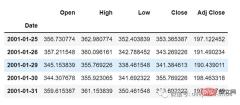

df.tail()

Now let’s take a moment to look at the data: The csv file contains Google’s stock data from 2001-01-25 to 2021-09-29. The data is based on day frequency.

[You can convert the frequency to "B" [weekday] or "D" if you want, since we won't be using dates, I'm just keeping it as it is. ]

Here we are trying to predict the future value of the "Open" column, so "Open" is the target column here.

Let’s take a look at the shape of the data:

df.shape
(5203,5)

Now let’s do the train-test split. Here we cannot shuffle the data as it must be sequential in time series.

test_split=round(len(df)*0.20)
df_for_training=df[:-1041]
df_for_testing=df[-1041:]
print(df_for_training.shape)
print(df_for_testing.shape)
(4162, 5)
(1041, 5)

It can be noticed that the data range is very large and they are not scaled in the same range, so to avoid prediction errors, let us first scale the data using MinMaxScaler. (You can also use StandardScaler)

scaler = MinMaxScaler(feature_range=(0,1))
df_for_training_scaled = scaler.fit_transform(df_for_training)
df_for_testing_scaled=scaler.transform(df_for_testing)
df_for_training_scaled

Split the data into X and Y, this is the most important part, read every step correctly.

def createXY(dataset,n_past):
 dataX = []
 dataY = []
 for i in range(n_past, len(dataset)):
 dataX.append(dataset[i - n_past:i, 0:dataset.shape[1]])
 dataY.append(dataset[i,0])
 return np.array(dataX),np.array(dataY)
trainX,trainY=createXY(df_for_training_scaled,30)
testX,testY=createXY(df_for_testing_scaled,30)

Let’s see what is done in the code above:

N_past is the number of steps in the past that we will look at when predicting the next target value.

Using 30 here means that the past 30 values ​​(all features including the target column) will be used to predict the 31st target value.

因此，在trainX中我们会有所有的特征值，而在trainY中我们只有目标值。

让我们分解for循环的每一部分：

对于训练，dataset = df_for_training_scaled, n_past=30

当i= 30：

data_X.addend (df_for_training_scaled[i - n_past:i, 0:df_for_training.shape[1]])

从n_past开始的范围是30，所以第一次数据范围将是-[30 - 30,30,0:5] 相当于 [0:30,0:5]

因此在dataX列表中，df_for_training_scaled[0:30,0:5]数组将第一次出现。

现在, dataY.append(df_for_training_scaled[i,0])

i = 30，所以它将只取第30行开始的open(因为在预测中，我们只需要open列，所以列范围仅为0，表示open列)。

第一次在dataY列表中存储df_for_training_scaled[30,0]值。

所以包含5列的前30行存储在dataX中，只有open列的第31行存储在dataY中。然后我们将dataX和dataY列表转换为数组，它们以数组格式在LSTM中进行训练。

我们来看看形状。

print("trainX Shape-- ",trainX.shape)
print("trainY Shape-- ",trainY.shape)
(4132, 30, 5)
(4132,)
print("testX Shape-- ",testX.shape)
print("testY Shape-- ",testY.shape)
(1011, 30, 5)
(1011,)

4132 是 trainX 中可用的数组总数，每个数组共有 30 行和 5 列， 在每个数组的 trainY 中，我们都有下一个目标值来训练模型。

让我们看一下包含来自 trainX 的 (30,5) 数据的数组之一 和 trainX 数组的 trainY 值：

print("trainX[0]-- n",trainX[0])
print("trainY[0]-- ",trainY[0])

如果查看 trainX[1] 值，会发现到它与 trainX[0] 中的数据相同（第一列除外），因为我们将看到前 30 个来预测第 31 列，在第一次预测之后它会自动移动 到第 2 列并取下一个 30 值来预测下一个目标值。

让我们用一种简单的格式来解释这一切：

trainX — — →trainY
[0 : 30,0:5] → [30,0]
[1:31, 0:5] → [31,0]
[2:32,0:5] →[32,0]

像这样，每个数据都将保存在 trainX 和 trainY 中。

现在让我们训练模型，我使用 girdsearchCV 进行一些超参数调整以找到基础模型。

def build_model(optimizer):
 grid_model = Sequential()
 grid_model.add(LSTM(50,return_sequences=True,input_shape=(30,5)))
 grid_model.add(LSTM(50))
 grid_model.add(Dropout(0.2))
 grid_model.add(Dense(1))
grid_model.compile(loss = 'mse',optimizer = optimizer)
 return grid_modelgrid_model = KerasRegressor(build_fn=build_model,verbose=1,validation_data=(testX,testY))
parameters = {'batch_size' : [16,20],
 'epochs' : [8,10],
 'optimizer' : ['adam','Adadelta'] }
grid_search = GridSearchCV(estimator = grid_model,
 param_grid = parameters,
 cv = 2)

如果你想为你的模型做更多的超参数调整，也可以添加更多的层。但是如果数据集非常大建议增加 LSTM 模型中的时期和单位。

在第一个 LSTM 层中看到输入形状为 (30,5)。它来自 trainX 形状。

(trainX.shape[1],trainX.shape[2]) → (30,5)

现在让我们将模型拟合到 trainX 和 trainY 数据中。

grid_search = grid_search.fit(trainX,trainY)

由于进行了超参数搜索，所以这将需要一些时间来运行。

你可以看到损失会像这样减少：

现在让我们检查模型的最佳参数。

grid_search.best_params_
{‘batch_size’: 20, ‘epochs’: 10, ‘optimizer’: ‘adam’}

将最佳模型保存在 my_model 变量中。

my_model=grid_search.best_estimator_.model

现在可以用测试数据集测试模型。

prediction=my_model.predict(testX)
print("predictionn", prediction)
print("nPrediction Shape-",prediction.shape)

testY 和 prediction 的长度是一样的。现在可以将 testY 与预测进行比较。

但是我们一开始就对数据进行了缩放，所以首先我们必须做一些逆缩放过程。

scaler.inverse_transform(prediction)

报错了，这是因为在缩放数据时，我们每行有 5 列，现在我们只有 1 列是目标列。

所以我们必须改变形状来使用 inverse_transform：

prediction_copies_array = np.repeat(prediction,5, axis=-1)

5 列值是相似的，它只是将单个预测列复制了 4 次。所以现在我们有 5 列相同的值 。

prediction_copies_array.shape
(1011,5)

这样就可以使用 inverse_transform 函数。

pred=scaler.inverse_transform(np.reshape(prediction_copies_array,(len(prediction),5)))[:,0]

但是逆变换后的第一列是我们需要的，所以我们在最后使用了 → [:,0]。

现在将这个 pred 值与 testY 进行比较，但是 testY 也是按比例缩放的，也需要使用与上述相同的代码进行逆变换。

original_copies_array = np.repeat(testY,5, axis=-1)
original=scaler.inverse_transform(np.reshape(original_copies_array,(len(testY),5)))[:,0]

现在让我们看一下预测值和原始值：

print("Pred Values-- " ,pred)
print("nOriginal Values-- " ,original)

最后绘制一个图来对比我们的 pred 和原始数据。

plt.plot(original, color = 'red', label = 'Real Stock Price')
plt.plot(pred, color = 'blue', label = 'Predicted Stock Price')
plt.title('Stock Price Prediction')
plt.xlabel('Time')
plt.ylabel('Google Stock Price')
plt.legend()
plt.show()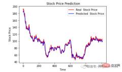

看样子还不错，到目前为止，我们训练了模型并用测试值检查了该模型。现在让我们预测一些未来值。

从主 df 数据集中获取我们在开始时加载的最后 30 个值[为什么是 30？因为这是我们想要的过去值的数量，来预测第 31 个值]

df_30_days_past=df.iloc[-30:,:]
df_30_days_past.tail()

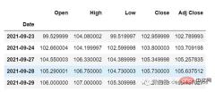
可以看到有包括目标列（“Open”）在内的所有列。现在让我们预测未来的 30 个值。

在多元时间序列预测中，需要通过使用不同的特征来预测单列，所以在进行预测时我们需要使用特征值（目标列除外）来进行即将到来的预测。

这里我们需要“High”、“Low”、“Close”、“Adj Close”列的即将到来的 30 个值来对“Open”列进行预测。

df_30_days_future=pd.read_csv("test.csv",parse_dates=["Date"],index_col=[0])
df_30_days_future

剔除“Open”列后，使用模型进行预测之前还需要做以下的操作：

缩放数据，因为删除了‘Open’列，在缩放它之前，添加一个所有值都为“0”的Open列。

缩放后，将未来数据中的“Open”列值替换为“nan”

现在附加 30 天旧值和 30 天新值（其中最后 30 个“打开”值是 nan）

df_30_days_future["Open"]=0
df_30_days_future=df_30_days_future[["Open","High","Low","Close","Adj Close"]]
old_scaled_array=scaler.transform(df_30_days_past)
new_scaled_array=scaler.transform(df_30_days_future)
new_scaled_df=pd.DataFrame(new_scaled_array)
new_scaled_df.iloc[:,0]=np.nan
full_df=pd.concat([pd.DataFrame(old_scaled_array),new_scaled_df]).reset_index().drop(["index"],axis=1)

full_df  形状是 (60,5)，最后第一列有 30 个 nan 值。

要进行预测必须再次使用 for 循环，我们在拆分 trainX 和 trainY 中的数据时所做的。但是这次我们只有 X，没有 Y 值。

full_df_scaled_array=full_df.values
all_data=[]
time_step=30
for i in range(time_step,len(full_df_scaled_array)):
 data_x=[]
 data_x.append(
 full_df_scaled_array[i-time_step :i , 0:full_df_scaled_array.shape[1]])
 data_x=np.array(data_x)
 prediction=my_model.predict(data_x)
 all_data.append(prediction)
 full_df.iloc[i,0]=prediction

对于第一个预测，有之前的 30 个值，当 for 循环第一次运行时它会检查前 30 个值并预测第 31 个“Open”数据。

当第二个 for 循环将尝试运行时，它将跳过第一行并尝试获取下 30 个值 [1:31] 。这里会报错错误因为Open列最后一行是 “nan”，所以需要每次都用预测替换“nan”。

最后还需要对预测进行逆变换：

new_array=np.array(all_data)
new_array=new_array.reshape(-1,1)
prediction_copies_array = np.repeat(new_array,5, axis=-1)
y_pred_future_30_days = scaler.inverse_transform(np.reshape(prediction_copies_array,(len(new_array),5)))[:,0]
print(y_pred_future_30_days)

这样一个完整的流程就已经跑通了。

如果你想看完整的代码，可以在这里查看：

​​https://www.php.cn/link/dd95829de39fe21f384685c07a1628d8​​

The above is the detailed content of Sales forecast using LSTM (Python code). For more information, please follow other related articles on the PHP Chinese website!