Richard Sutton bluntly stated that convolutional backpropagation has fallen behind, and AI breakthroughs require new ideas: continuous backpropagation

"Loss of Plasticity" is one of the most commonly criticized shortcomings of deep neural networks, which is also one of the reasons why AI systems based on deep learning are considered unable to continue learning.

For the human brain, "plasticity" refers to the ability to generate new neurons and new connections between neurons, which is an important basis for continuous learning. As we age, the brain's plasticity gradually decreases at the expense of consolidating what we have learned. Neural networks are similar.

An vivid example is that warm-starting training in 2020 was proven: only by discarding the initially learned content and learning the entire data in one go Only through intensive training can we achieve better learning results.

In deep reinforcement learning (DRL), the AI ​​system often has to "forget" all the content previously learned by the neural network, save only part of the content to the playback buffer, and then from Achieve continuous learning from scratch. This way of resetting the network is also considered to prove that deep learning cannot continue to learn.

So, how can we keep learning systems malleable?

Recently, Richard Sutton, the father of reinforcement learning, gave a speech titled "Maintaining Plasticity in Deep Continual Learning" at the CoLLAs 2022 conference, and proposed what he believed could solve this problem. Answer: Continuous Backpropagation algorithm (Continual Backprop).

Richard Sutton first proved the existence of plasticity loss from the perspective of the data set, then analyzed the causes of plasticity loss from within the neural network, and finally proposed the continuous backpropagation algorithm as Ways to solve the loss of plasticity: Reinitialize a small number of neurons with low utility. This continuous injection of diversity can maintain the plasticity of deep networks indefinitely.

The following is the full text of the speech, which has been compiled by AI Technology Review without changing the original meaning.

1 The real existence of plasticity loss

Can deep learning really solve the problem of continuous learning?

The answer is no, mainly for the following three points:

1. "Unsolvable" refers to non-depth linear Network, the learning speed will eventually be very slow;
2. The professional standardized methods used in deep learning are only effective in one-time learning and are contrary to continuous learning;
3. Replay caching itself is an extreme way to admit that deep learning is not feasible.

Therefore, We must find better algorithms suitable for this new learning model and get rid of the limitations of one-time learning.

First, we used the ImageNet and MNIST data sets for classification tasks, implemented regression prediction, and directly tested the continuous learning effect, proving the existence of plasticity loss in supervised learning.

ImageNet Dataset Test

ImageNet is a dataset containing millions of images tagged with nouns. It has 1000 categories with 700 or more images per category and is widely used for category learning and category prediction.

Below is a photo of a shark, downsampled to 32*32 size. The purpose of this experiment is to find minimal changes from deep learning practices. We divided the 700 images of each category into 600 training samples and 100 test samples, and then divided the 1000 categories into two groups to generate a binary classification task sequence with a length of 500. All data sets were randomly mess up the order. After training for each task, we evaluate the accuracy of the model on the test sample, run it 30 times independently and take the average before entering the next binary classification task.

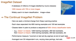
500 classification tasks will share the same network. In order to eliminate the impact of complexity, the head network will be reset after task switching. We use a standard network, that is, 3 layers of convolution and 3 layers of fully connected, but the output layer may be relatively small for the ImageNet dataset because only two categories are used for one task. For each task, every 100 examples are taken as a batch, with a total of 12 batches and 250 epochs of training. Only one initialization is performed before starting the first task, using the Kaiming distribution to initialize the weights. A momentum-based stochastic gradient descent method is used for the cross-entropy loss, and a ReLU activation function is used.

Two questions arise here:

1. How will performance evolve in the task sequence?

2. On which task will the performance be better? Is the initial first mission better? Or will subsequent tasks benefit from the experience of previous tasks?

The following figure gives the answer, The performance of continuous learning is comprehensively determined by the training step size and backpropagation.

Since it is a binary classification problem, the chance probability is 50%, and the shaded area represents the standard deviation, which is not significant. The linear benchmark uses a linear layer to directly process pixel values, which is not as effective as the deep learning method. This difference is significant.

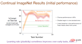
Note: Using a smaller learning rate (α=0.001) will result in higher accuracy, in the first 5 tasks Performance gradually improves, but tends to decline in the long run.

We then increased the number of tasks to 2000 and further analyzed the impact of the learning rate on the continuous learning effect. The accuracy was calculated on average every 50 tasks. The result is shown below.

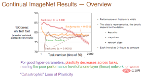
Legend: The accuracy of the red curve with α=0.01 on the first task is about 89%. Once the number of tasks Beyond 50, the accuracy decreases. As the number of tasks further increases, plasticity gradually loses, and the final accuracy is lower than the linear baseline. When α=0.001, the learning speed slows down, the plasticity also decreases sharply, and the accuracy is only a little higher than the linear network.

Therefore, for good hyperparameters, the plasticity between tasks will decay and the accuracy will be lower than using only one layer of neural network. The red curve shows almost It’s a “catastrophic loss of plasticity.”

The training results also depend on parameters such as the number of iterations, the number of steps, and the network size. The training time for each curve in the figure is 24 hours on multiple processors. When doing the system It may not be practical in sexual experiments, so we next choose the MNIST data set for testing.

MNIST Data Set Test

The MNIST data set contains a total of 60,000 handwritten digit images, with 10 categories from 0 to 9, and are 28*28 grayscale images. .

Goodfellow et al. once created a new test task by shuffling the order or randomly arranging pixels. The image in the lower right corner is an example of the generated arranged image. We adopt this method. To generate the entire task sequence, 6000 images are presented in a random manner in each task. No task content is added here, and the network weights are only initialized once before the first task. We can use online cross-entropy loss for training, and continue to use the accuracy index to measure the effect of continuous learning.

The neural network structure is 4 fully connected layers, the number of neurons in the first 3 layers is 2000, and the number of neurons in the last layer is 10. Since the images of the MNIST dataset are centered and scaled, no convolution operations are performed. All classification tasks share the same network, using stochastic gradient descent without momentum, and other settings are the same as those tested on the ImageNet dataset.

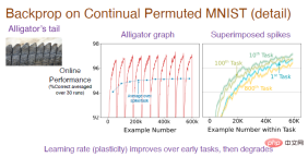
Note: The middle picture is the result of running the task sequence 30 times independently and taking the average. Each task has 6000 samples. Since it is a classification task, the random guess at the beginning is accurate. The rate is 10%. After the model learns the rules of arranging images, the prediction accuracy will gradually increase. However, after switching tasks, the accuracy drops to 10%, so the overall trend is constantly fluctuating. The picture on the right shows the learning effect of the model on each task. The initial accuracy is 0. Over time, the effect gradually gets better. The accuracy on the 10th task is better than the 1st task, but the accuracy drops on the 100th task, and the accuracy on the 800th task is even lower than the first one.

In order to understand the whole process, we need to focus on analyzing the accuracy of the convex part, and then average it to get the blue curve of the intermediate image. It can be clearly seen that the accuracy will gradually increase at the beginning and then level off until the 100th task. So why does the accuracy drop sharply at the 800th task?

Next, we tried different step values ​​on more task sequences to further observe their learning effects. The results are as follows:

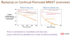
Note: The red curve uses the same step value as the previous experiment, and the accuracy is indeed declining steadily. The plasticity loss is relatively large.

#At the same time, the greater the learning rate, the faster the plasticity decreases. There is a huge plasticity loss for all step size values. In addition, the number of neurons in the hidden layer will also affect the accuracy. The number of neurons in the brown curve is 10,000. Due to the enhanced fitting ability of the neural network, the accuracy will drop very slowly at this time, and there will still be a loss of plasticity. However, the larger the network size, The smaller the size, the faster the plasticity decreases.

So from inside the neural network, why is there a loss of plasticity?

The picture below explains why. It can be found that the excessive number of "dead" neurons, the excessive weight of neurons, and the loss of neuronal diversity are all causes of plasticity loss.

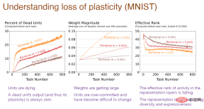
Note: The horizontal axis still represents the task number, and the vertical axis of the first picture represents the "death" nerve Percentage of neurons, "dead" neurons are neurons whose output and gradient are always 0 and no longer predict the plasticity of the network. The vertical axis of the second graph represents the weight. The vertical axis of the third graph represents the effective level of the number of remaining hidden neurons.

2 Limitations of existing methods

We analyzed whether existing deep learning methods other than backpropagation Will help maintain plasticity.

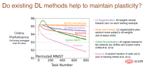
The results show that the L2 regularization method will reduce the plasticity loss, reducing the weight to 0 in the process, so that it can be dynamically adjusted and Stay malleable.

The shrinkage and perturbation methods are similar to L2 regularization, but also add random noise to all weights to increase diversity, with basically no loss of plasticity.

We also tried other online standardization methods, which worked relatively well at the beginning, but the plasticity loss was serious as learning continued. The performance of the Dropout method is even worse. We randomly set a part of the neurons to 0 for retraining and found that the plasticity loss increased sharply.

Various methods will also have an impact on the internal structure of the neural network. Using a regularization method will increase the percentage of "dead" neurons, because in the process of shrinking the weights to 0, if they stay at 0, it will cause the output to be 0 and the neurons will "die". And shrinkage and perturbation add random noise to the weights, so there aren't too many "dead" neurons. The normalization method also has a lot of "dead" neurons and it seems to be going in the wrong direction, and Dropout is similar.

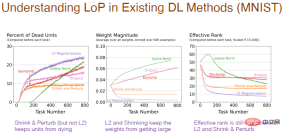
The result of the weight changing with the number of tasks is more reasonable. Using regularization will obtain a very small weight. Shrinkage and perturbation add noise on the basis of regularization, and the decrease in weight is relatively weakened. Standardization will increase the weight. However, for L2 regularization, contraction and perturbation, the effective level of the number of hidden neurons is relatively low, indicating that its performance in maintaining diversity is poor, which is also a problem.

Slowly changing regression problem (SCR)

All our ideas and algorithms are derived from Slowly changing regression problemExperiments, this is A new idealized question focused on continuous learning.

In this experiment, our purpose is to achieve an objective function formed by a single-layer neural network with random weights, and the hidden layer neurons are 100 linear threshold neurons.

We did not do classification, we just generated a number, so this is a regression problem. Every 10,000 training steps, we select 1 bit from the last 15 bits of the input to flip, so this is a slowly changing objective function.

Our solution is touse the same network structure, containing only one hidden layer of neurons, while ensuring that the activation function is differentiable, but we will have 5 hidden layers Neurons. This is similar to RL. The range of exploration by the agent is much smaller than the interactive environment, so it can only perform approximate processing. As the objective function changes, try to change the approximate value, which will make it easier to do some systematic experiments.

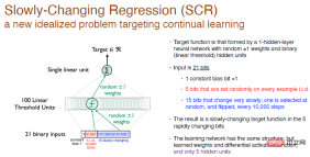
Legend: The input is a 21-bit random binary number. The first bit is the input constant deviation with a value of 1, and the middle 5 bits are independent and identically distributed random numbers, the other 15 bits are slowly changing constants, and the output is a real number. The weights are randomized to 0 and can be randomly chosen to be 1 or -1.

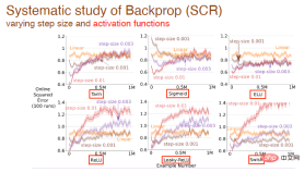
We further studied the impact of changing step values ​​and activation functions on the learning effect. For example, tanh, sigmoid and relu activation functions are used here:

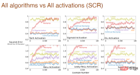
and the influence of activation function form on the learning effect of all algorithms:

When the step size and activation function change at the same time, we also made a systematic analysis of the impact of Adam backpropagation:

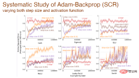
Finally: After using different activation functions, the error changes between different algorithms based on the Adam mechanism:

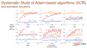
The above experimental results show that deep learning The method is no longer suitable for continuous learning. When encountering new problems, the learning process will become very slow and the advantage of depth will not be reflected. Standardized methods in deep learning are only suitable for one-time learning. We need to improve deep learning methods to make it possible to use them for continuous learning.

3 Continuous Backpropagation

Will the convolutional backpropagation algorithm itself be a good continuous learning algorithm?

We think not.

The convolution backpropagation algorithm mainly contains two aspects: initialization with small random weights and gradient descent at each time step. Although it generates small random numbers at the beginning to initialize the weights, it does not repeat again. Ideally, we might want some learning algorithm that can perform similar computations at any time.

So how do we make the convolutional backpropagation algorithm learn continuously?

The simplest way is to selectively reinitialize, such as initializing after performing several tasks. But at the same time, reinitializing the entire network may not be reasonable in continuous learning, because it means that the neural network is forgetting everything it has learned. So we'd better selectively initialize part of the neural network, such as reinitializing some "dead" neurons, or sorting the neural network according to utility and reinitializing neurons with lower utility.

The idea of ​​random selection initialization is related to the generation and testing method proposed by Mahmood and Sutton in 2012. It only needs to generate some neurons and test their practicality, and the continuous backpropagation algorithm is built bridge between these two concepts. The generation and testing method has some limitations, using only one hidden layer and only one output neuron, we extend it to a multi-layer network that can be optimized with some deep learning methods.

We first considersetting the network into multiple layers instead of a single output. Previous work mentioned the concept of utility. Since there is only one weight, this utility is only a weight-level concept. However, we have multiple weights. The simplest generalization is to consider utility at the weight summation level.

Another idea is to consider the activity of the features instead of just the output weights, so we can multiply the sum of the weights by the average feature activation function, thus Allocate different proportions. We hope to design algorithms that can continue to learn and keep running fast. We also consider the plasticity of features when calculating utility. Finally, the average contribution of features is transferred to the output bias, reducing the impact of feature deletion.

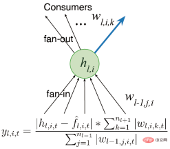
There are two main directions for future improvements: (1) We need toglobally measure utility and measure neural The influence of elements on the entire function represented is not limited to local measures such as input weights, output weights and activation functions; (2) We need to furtherimprove the generator,currently only from the initial distribution Sampling is performed for initialization, and initialization methods that can improve performance are also explored.

So, how well does continuous backpropagation perform in maintaining plasticity?

Experimental results show that continuous backpropagation is trained using the online arranged MNIST data set, and fully maintains plasticity. The blue curve in the figure below shows this result.

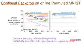
Note: The picture on the right shows the impact of different replacement rates on continuous learning. For example, the replacement rate of 1e-6 means that every time steps to replace 1/1000000 representations. That is, assuming there are 2000 features, one neuron will be replaced in each layer every 500 steps. This update speed is very slow, so the replacement rate is not very sensitive to hyperparameters and will not significantly affect the learning effect.

Next, we need to study the impact of continuous backpropagation on the internal structure of the neural network. Continuous back propagation has almost no "dead" neurons, Because the utility considers the average feature activation, if a neuron "dies", it will be replaced immediately. And because we keep replacing neurons, we get new neurons with smaller weight magnitudes. Because neurons are randomly initialized, they accordingly retain richer representations and diversity.

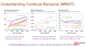
Therefore, continuous backpropagation solves all the problems caused by the lack of plasticity on the MNIST dataset.

So, can continuous backpropagation be extended to deeper convolutional neural networks?

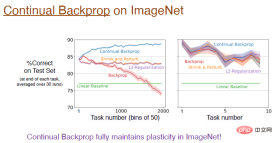
The answer is yes! On the ImageNet dataset, continuous backpropagation fully preserved plasticity, and the model's final accuracy was around 89%. In fact, in the initial training stage, the performance of these algorithms is equivalent. As mentioned earlier, the replacement rate changes very slowly, and the approximation is better only when the number of tasks is large enough.

Here we take the "Slippery Ant" problem as an example to show the experimental results of a reinforcement learning.

The "Slippery Ant" problem is an extension of the non-stationary reinforcement problem and is basically similar to the PyBullet environment. The only difference is that the friction between the ground and the agent increases every 10 million steps. changes occur. We implemented a continuous learning version of the PPO algorithm based on continuous backpropagation, which can be selectively initialized. The comparison results between the PPO algorithm and the continuous PPO algorithm are as follows.

Note: The PPO algorithm performed well at the beginning, but as the training progressed, the performance continued to decline. The L2 algorithm and shrinkage were introduced. and perturbation algorithm will be alleviated. The continuous PPO algorithm performed relatively well, retaining most of the plasticity.

What’s interesting is that the agent trained by the PPO algorithm can only struggle to walk, but the agent trained by the PPO algorithm continuously can run very far.

4 Conclusion

Deep learning networks are mainly optimized for one-time learning. In a sense, they may be completely useless for continuous learning. fail. Deep learning methods like normalization and DropOut may not be helpful for continuous learning, but making some small improvements on this basis, such as continuous backpropagation, can be very effective.

Continuous backpropagation sorts network features according to the utility of neurons. Especially for recurrent neural networks, there may be more improvements to the sorting method.

Reinforcement learning algorithms utilize the idea of ​​policy iteration. Although continuous learning problems exist, maintaining the plasticity of deep learning networks opens up huge new possibilities for RL and model-based RL.

The above is the detailed content of Richard Sutton bluntly stated that convolutional backpropagation has fallen behind, and AI breakthroughs require new ideas: continuous backpropagation. For more information, please follow other related articles on the PHP Chinese website!