Home >Common Problem >How to add pictures to Excel worksheet cells
How to add pictures to Excel worksheet cells
- WBOYWBOYWBOYWBOYWBOYWBOYWBOYWBOYWBOYWBOYWBOYWBOYWBforward
- 2023-04-17 11:49:0519507browse
You may be wondering if you have the option to add any image or photo to an Excel spreadsheet cell? Well, most users don't know how to do it, or if it has any functionality. But once you add or insert an image in your spreadsheet, it's not that easy to fit it into the cells.
Even after adding the image, it can become a problem if any operations involving specific cells in rows or columns are required. If you also find it difficult to add or insert images in spreadsheet cells or use it while using any formula or operation, then this article will guide you on how to do it easily by following the steps below.
How to add pictures to Excel worksheet cells
Step 1: First press the Windows key on the keyboard, and then enter excel.
Step 2: After that, select Excel application from the search results to open the Excel application on your system as shown in the below screen As shown in the screenshot.

Step 3: Next, you can click Blank Workbook or open any other existing save from your computer by browsing The Excel worksheet is as shown below.

Step 4: Once the spreadsheet is open, to add images to the worksheet, you need to go to the Insert tab on the top bar.
Step 5: Then, click on the Image option in the Illustrations section and select This device from the drop-down menu as shown in the screenshot below shown.
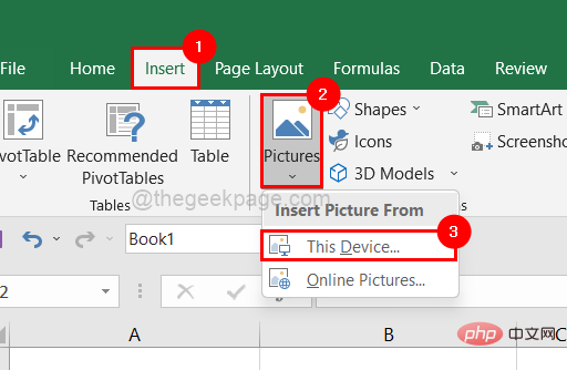
Step 6: In the Insert Picture window, browse to the folder containing your images and select as many images as you want, then click on the Insert" as shown below.
Note: In this example, we have selected two pictures, you can choose one or more you want.

Step 7: After adding the image to the worksheet, to fit the image to a specific cell, you need to hold down the ALT key on your keyboard Drag the edges of the image.
Note: The screenshot below shows what it will look like after inserting the image into the cell.
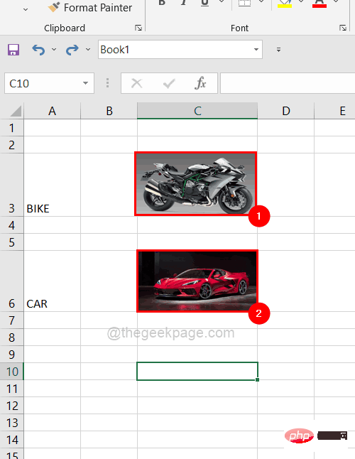
Step 8: Now select any row that contains the image you just inserted.

Step 9: Right-click on the row and click on the Hide option from the context menu as shown below.
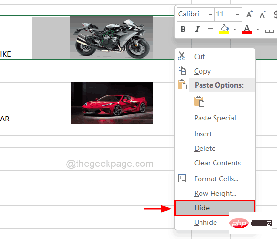
Step 10: If you observe that the row is hidden but the image is not hidden along with the row.

Step 11: So to make the image move with the cell, first select only the image of a specific row.
Step 12: Then, right-click on the image and click "Format Image " from the menu, as shown below.
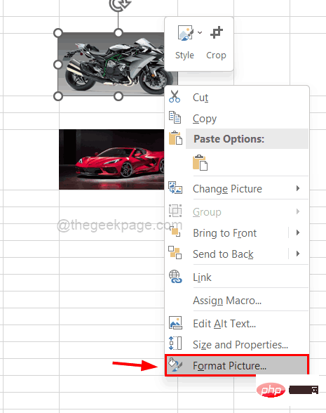
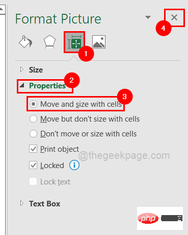
#Step 13: On the right side, a small window to format the picture appears.
Step 14: Go to the Size and Properties icon on the top menu as shown below.
Step 15: Then, click Properties to expand it so you can view the options.
Step 16: Now select the "Move and resize cells" radio button from the list and then close the "Format Picture" window as shown in the image.
Step 17: Now, if you try to hide the row, you can see that the entire row is hidden as well as the image inserted into the cell of the row.

Step 18: Now you need to do the same thing one by one for all the images inserted into the Excel table cells.
The above is the detailed content of How to add pictures to Excel worksheet cells. For more information, please follow other related articles on the PHP Chinese website!

