 Technology peripherals
 AI
AI Single GPU realizes 20Hz online decision-making, interpretation of the latest efficient trajectory planning method based on sequence generation model
Single GPU realizes 20Hz online decision-making, interpretation of the latest efficient trajectory planning method based on sequence generation model
Previously we introduced the application of sequence modeling methods based on Transformer and Diffusion Model in reinforcement learning, especially in the field of offline continuous control. Among them, Trajectory Transformer (TT) and Diffusser are model-based planning algorithms. They show very high-precision trajectory prediction and good flexibility, but the decision-making delay is relatively high. In particular, TT discretizes each dimension independently as a symbol in the sequence, which makes the entire sequence very long, and the time consumption of sequence generation will increase rapidly as the dimensions of states and actions increase.
In order to enable the trajectory generation model to achieve practical level decision-making speed, we started the project of efficient trajectory generation and decision-making in parallel with Diffusser (overlapping but should be later) . Our first thought was to fit the entire trajectory distribution with a Transformer Mixture of Gaussian in continuous space rather than a discrete distribution. Although implementation problems are not ruled out, we have not been able to obtain a relatively stable generation model under this approach. Then we tried Variational Autoencoder (VAE) and made some breakthroughs. However, the reconstruction accuracy of VAE is not particularly ideal, making the downstream control performance quite different from that of TT. After several rounds of iterations, we finally selected VQ-VAE as the basic model for trajectory generation, and finally obtained a new algorithm that can efficiently sample and plan, and performs far better than other model-based methods on high-dimensional control tasks. We Called Trajectory Autoencoding Planner (TAP).
- ## Project homepage: https://sites.google .com/view/latentplan
- Paper homepage: https://arxiv.org/abs/2208.10291
Under a single GPU, TAP can easily make online decisions with a decision-making efficiency of 20Hz. In the low-dimensional D4RL task, the decision-making delay is only TT Around 1%. What's more important is that as the task state and action dimension D increase, the theoretical decision delay of TT will grow with the cubic power , and the Diffusser will theoretically grow linearly
 , while TAP’s decision-making speed is not affected by dimensions
  . In terms of the agent's decision-making performance, as the action dimension increases, TAP's performance improves compared to other methods, and the improvement compared to model-based methods (such as TT) is particularly obvious.
The importance of decision delay to decision-making and control tasks is very obvious. Although algorithms like MuZero perform well in simulation environments, they require real-time and rapid response in the real world. task, excessive decision-making delay will become a major difficulty in its deployment. In addition, under the premise of having a simulation environment, the slow decision-making speed will also lead to high testing costs for similar algorithms, and the cost of being used in online reinforcement learning will also be relatively high.
In addition, we believe that allowing the sequence generation modeling method to be smoothly extended to tasks with higher dimensions is also a very important contribution of TAP. In the real world, most of the problems we hope reinforcement learning can ultimately solve actually have higher state and action dimensions. For example, for autonomous driving, the inputs from various sensors are unlikely to be less than 100 even after preprocessing at various perceptual levels. Complex robot control often also has a high action space. The degrees of freedom of all human joints are about 240, which corresponds to an action space of at least 240 dimensions. A robot as flexible as a human also requires an equally high-dimensional action space.
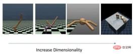
Four sets of tasks with gradually increasing dimensions
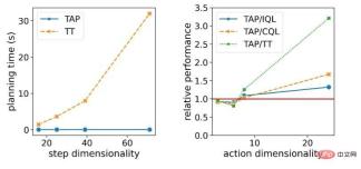
Changes in decision latency and relative model performance as task dimensions grow
Method Overview
First, train the autoencoder (autoencoders) part of VQ-VAE. There are two differences from the original VQ-VAE. The first difference is that both the encoder and decoder are based on Causal Transformer instead of CNN. The second difference is that we learn a conditional probability distribution, and the possible trajectories being modeled must all start from the current state  . The autoencoder learns a bidirectional mapping between trajectories starting from the current state
  and latent codes. These latent codes are arranged in chronological order like the original trajectories, and each latent code will be mapped to the actual
  step trajectory. Because we use Causal Transformer, latent codes with lower temporal ranking (such as
  ) will not transmit information to sequences with higher temporal ranking (such as
  ), which allows TAP to decode a trajectory of length NL through the first N hidden coding parts, which is very useful when using it for subsequent planning.
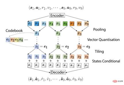
We will then use another GPT-2-style Transformer to model the conditional probability distribution of these latent codes  :
:
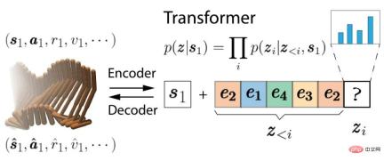
When making decisions, we can find the best future trajectory by optimizing within the latent variable space, rather than in the original action space optimize. A very simple but effective method is to sample directly from the latent coding distribution, and then select the best-performing trajectory, as shown below:

The objective score referenced when selecting the optimal trajectory will consider both the expected return of the trajectory (reward plus the valuation of the last step) and the feasibility or probability of the trajectory itself. Such as the following formula, where  is a number much larger than the highest return. When the probability of the trajectory is higher than a threshold
  , the standard for judging this trajectory will be Its expected return (highlighted in red), otherwise the probability of this trajectory itself would be the dominant component (highlighted in blue). In other words, TAP will select the one with the highest expected return among the trajectories greater than the threshold.

Although the number of samples is large enough, direct sampling can also be very effective when the prediction sequence is short. Under the premise of limiting the number of samples and the total time required for planning, it is better to use a better optimizer. will lead to better performance. The following two animations show the difference between trajectories generated by direct sampling and beam search when predicting 144 steps into the future. These trajectories are sorted by the final target score. The trajectories at the top of the top layer have higher scores, and the trajectories stacked behind them have lower scores. In addition, trajectories with low scores will also have lower transparency.
In the picture we can see that many of the dynamics of the trajectories generated by direct sampling are unstable and do not conform to physical laws. In particular, the lighter trajectories in the background are almost all floating. Go. These are all trajectories with relatively low probability and will be eliminated when the final plan is selected. The trajectory in the front row looks more dynamic, but the corresponding performance is relatively poor, and it seems like it is about to fall. In contrast, beam search will dynamically consider the probability of the trajectory when expanding the next hidden variable, so that branches with very low probability will be terminated early, so that the candidate trajectories generated will focus on those with better performance and possibility. The larger tracks are around.

Direct sampling

##Beam search
Experimental resultsIn the absence of more advanced valuation and strategy improvement, relying solely on the advantage of prediction accuracy, in On low-dimensional tasks, TAP has achieved comparable performance to other offline reinforcement learning:
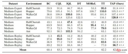
gym locomotion control
On high-dimensional tasks, TAP has achieved far better performance than other model-based methods, and also outperformed common model-free methods. There are actually two open questions that have not yet been answered. The first is why previous model-based methods performed poorly in these high-dimensional offline reinforcement learning tasks, and the second is why TAP can outperform many model-free methods on these tasks. One of our assumptions is that it is very difficult to optimize a policy on a high-dimensional problem while also taking into account preventing the policy from deviating too much from the behavioral policy. When a model is learned, errors in the model itself may amplify this difficulty. TAP moves the optimization space to a small discrete hidden variable space, which makes the entire optimization process more robust.
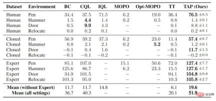
##adroit robotic hand controlSome slice studies
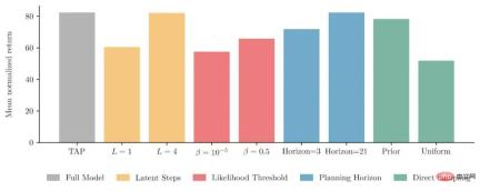
For many designs in TAP, we have also done a series of slice studies on the task of gym locomotion control. The first is the number of steps of the trajectory that each latent code actually corresponds to (yellow histogram). Facts have proved that allowing a latent variable to correspond to multi-step state transitions not only has computational advantages, but also has good performance in the final model. There has also been an improvement. By adjusting the threshold that triggers low-probability trajectory penalties in the search objective function Finally we tried the performance of TAP under direct sampling (green histogram). Note that the number of samples sampled here is 2048, while the number in the above animation is only 256, and the above animation generates a plan for the next 144 steps, but in fact our basic model directs planning for 15 steps. The conclusion is that direct sampling can achieve similar performance to beam search if the number of samples is sufficient and the planning path is not long. But this is a case of sampling from the learned conditional distribution of latent variables. If we directly sample with equal probability from the latent coding, it will still be much worse than the complete TAP model in the end. Results of Slice Study (red histogram), we also confirmed that both parts of the objective function are indeed helpful to the final performance of the model. Another point is that the number of steps planned into the future (planning horizon, blue histogram) has little impact on model performance. In the post-deployment search, even if only one latent variable is expanded, the final agent's performance will only be reduced by 10%. about.
The above is the detailed content of Single GPU realizes 20Hz online decision-making, interpretation of the latest efficient trajectory planning method based on sequence generation model. For more information, please follow other related articles on the PHP Chinese website!
 What is Graph of Thought in Prompt EngineeringApr 13, 2025 am 11:53 AM
Introduction In prompt engineering, “Graph of Thought” refers to a novel approach that uses graph theory to structure and guide AI’s reasoning process. Unlike traditional methods, which often involve linear s
 Optimize Your Organisation's Email Marketing with GenAI AgentsApr 13, 2025 am 11:44 AM
Introduction Congratulations! You run a successful business. Through your web pages, social media campaigns, webinars, conferences, free resources, and other sources, you collect 5000 email IDs daily. The next obvious step is
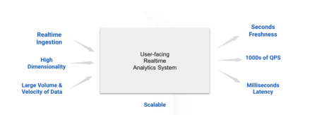 Real-Time App Performance Monitoring with Apache PinotApr 13, 2025 am 11:40 AM
Introduction In today’s fast-paced software development environment, ensuring optimal application performance is crucial. Monitoring real-time metrics such as response times, error rates, and resource utilization can help main
 ChatGPT Hits 1 Billion Users? 'Doubled In Just Weeks' Says OpenAI CEOApr 13, 2025 am 11:23 AM
“How many users do you have?” he prodded. “I think the last time we said was 500 million weekly actives, and it is growing very rapidly,” replied Altman. “You told me that it like doubled in just a few weeks,” Anderson continued. “I said that priv
 Pixtral-12B: Mistral AI's First Multimodal Model - Analytics VidhyaApr 13, 2025 am 11:20 AM
Introduction Mistral has released its very first multimodal model, namely the Pixtral-12B-2409. This model is built upon Mistral’s 12 Billion parameter, Nemo 12B. What sets this model apart? It can now take both images and tex
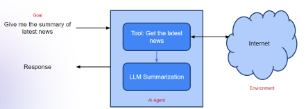 Agentic Frameworks for Generative AI Applications - Analytics VidhyaApr 13, 2025 am 11:13 AM
Imagine having an AI-powered assistant that not only responds to your queries but also autonomously gathers information, executes tasks, and even handles multiple types of data—text, images, and code. Sounds futuristic? In this a
 Applications of Generative AI in the Financial SectorApr 13, 2025 am 11:12 AM
Introduction The finance industry is the cornerstone of any country’s development, as it drives economic growth by facilitating efficient transactions and credit availability. The ease with which transactions occur and credit
 Guide to Online Learning and Passive-Aggressive AlgorithmsApr 13, 2025 am 11:09 AM
Introduction Data is being generated at an unprecedented rate from sources such as social media, financial transactions, and e-commerce platforms. Handling this continuous stream of information is a challenge, but it offers an


Hot AI Tools

Undresser.AI Undress
AI-powered app for creating realistic nude photos

AI Clothes Remover
Online AI tool for removing clothes from photos.

Undress AI Tool
Undress images for free

Clothoff.io
AI clothes remover

AI Hentai Generator
Generate AI Hentai for free.

Hot Article

Hot Tools

SublimeText3 Chinese version
Chinese version, very easy to use

mPDF
mPDF is a PHP library that can generate PDF files from UTF-8 encoded HTML. The original author, Ian Back, wrote mPDF to output PDF files "on the fly" from his website and handle different languages. It is slower than original scripts like HTML2FPDF and produces larger files when using Unicode fonts, but supports CSS styles etc. and has a lot of enhancements. Supports almost all languages, including RTL (Arabic and Hebrew) and CJK (Chinese, Japanese and Korean). Supports nested block-level elements (such as P, DIV),

DVWA
Damn Vulnerable Web App (DVWA) is a PHP/MySQL web application that is very vulnerable. Its main goals are to be an aid for security professionals to test their skills and tools in a legal environment, to help web developers better understand the process of securing web applications, and to help teachers/students teach/learn in a classroom environment Web application security. The goal of DVWA is to practice some of the most common web vulnerabilities through a simple and straightforward interface, with varying degrees of difficulty. Please note that this software

Dreamweaver Mac version
Visual web development tools

SecLists
SecLists is the ultimate security tester's companion. It is a collection of various types of lists that are frequently used during security assessments, all in one place. SecLists helps make security testing more efficient and productive by conveniently providing all the lists a security tester might need. List types include usernames, passwords, URLs, fuzzing payloads, sensitive data patterns, web shells, and more. The tester can simply pull this repository onto a new test machine and he will have access to every type of list he needs.


