
Home >Backend Development >Python Tutorial >Python implements 12 dimensionality reduction algorithms
Python implements 12 dimensionality reduction algorithms

- WBOYWBOYWBOYWBOYWBOYWBOYWBOYWBOYWBOYWBOYWBOYWBOYWBforward
- 2023-04-12 22:55:131815browse
Hello everyone, I am Peter~
The information on various dimensionality reduction algorithms on the Internet is uneven, and most of them do not provide source code. Here is a GitHub project that uses Python to implement 11 classic data extraction (data dimensionality reduction) algorithms, including: PCA, LDA, MDS, LLE, TSNE, etc., with relevant information and display effects; very suitable for machine learning Beginners and those who have just started data mining.
Why do we need to perform data dimensionality reduction?
The so-called dimensionality reduction is to use a set of vectors Zi with a number of d to represent the useful information contained in a vector Xi with a number of D, where d
Usually, we will find that the dimensions of most data sets will be hundreds or even thousands, and the dimensions of the classic MNIST are all 64.
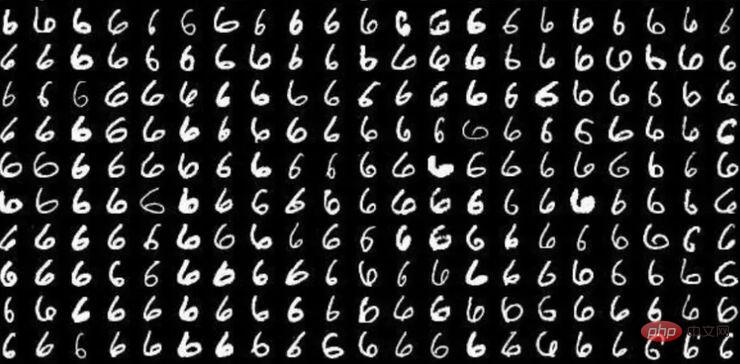
MNIST handwritten digit data set
But in actual applications, the useful information we use does not require such a high dimension, and every increase The number of samples required for one dimension increases exponentially, which may directly lead to a great "dimensionality disaster"; data dimensionality reduction can achieve:
- Make the data set easier to use
- Ensure that variables are independent of each other
- Reduce the cost of algorithm calculations
Remove noise Once we can correctly process this information and perform dimensionality reduction correctly and effectively, this It will greatly help reduce the amount of calculations and thus improve the efficiency of machine operation. Data dimensionality reduction is also often used in fields such as text processing, face recognition, image recognition, and natural language processing.
Principle of Data Dimensionality Reduction
Often data in high-dimensional space will be sparsely distributed, so during the process of dimensionality reduction, we usually do some data deletion. These data include Redundant data, invalid information, repeated expressions, etc. are eliminated.
For example: There is a 1024*1024 picture. Except for the 50*50 area in the center, all other positions have zero values. These zero information can be classified as useless information; for symmetrical graphics, The symmetrical part of the information can be classified as repeated information.
Therefore, most classic dimensionality reduction techniques are also based on this content. Dimensionality reduction methods are divided into linear and nonlinear dimensionality reduction. Nonlinear dimensionality reduction is divided into kernel function-based and eigenvalue-based. Methods.
- Linear dimensionality reduction method: PCA, ICA LDA, LFA, LPP (linear representation of LE)
- Nonlinear dimensionality reduction method:
Based on Nonlinear dimensionality reduction method of kernel function - KPCA, KICA, KDA
Nonlinear dimensionality reduction method based on eigenvalue (flow pattern learning) - ISOMAP, LLE, LE, LPP, LTSA, MVU
Heucoder, a master's student majoring in computer technology at Harbin Institute of Technology, compiled a total of 12 classic dimensionality reduction algorithms including PCA, KPCA, LDA, MDS, ISOMAP, LLE, TSNE, AutoEncoder, FastICA, SVD, LE, and LPP. Relevant information, codes and displays are provided. The following will mainly use the PCA algorithm as an example to introduce the specific operations of the dimensionality reduction algorithm.
Principal Component Analysis (PCA) dimensionality reduction algorithm
PCA is a mapping method based on mapping from high-dimensional space to low-dimensional space. It is also the most basic unsupervised dimensionality reduction algorithm. The goal is to project in the direction where the data changes the most, or in the direction where the reconstruction error is minimized. It was proposed by Karl Pearson in 1901 and is a linear dimensionality reduction method. The principles associated with PCA are often called maximum variance theory or minimum error theory. The two have the same goal, but the process focus is different.
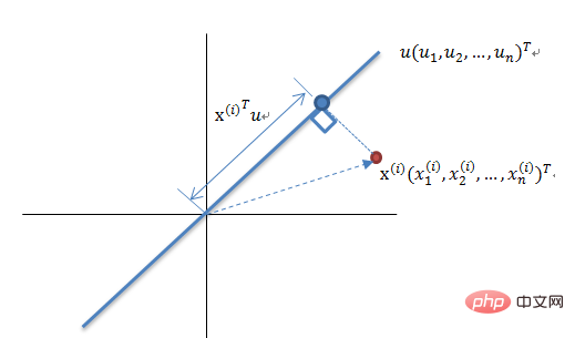
Maximum Variance Theory Dimensionality Reduction Principle
Reducing a set of N-dimensional vectors to K-dimensional (K greater than 0, less than N), the goal is to select There are K unit orthogonal bases, the COV(X,Y) of each field is 0, and the variance of the fields is as large as possible. Therefore, the maximum variance means that the variance of the projection data is maximized. In this process, we need to find the best projection space Wnxk, covariance matrix, etc. of the data set Xmxn. The algorithm flow is:
- Algorithm input: Data set Xmxn;
- Calculate the mean Xmean of the data set Denoted as Cov;
- Calculate the eigenvalues and corresponding eigenvectors of the covariance matrix COV;
- Sort the eigenvalues from large to small, select the largest k ones, and then The corresponding k eigenvectors are used as column vectors to form the eigenvector matrix Wnxk;
- Calculate XnewW, that is, project the data set Xnew onto the selected eigenvectors, thus obtaining the dimensionally reduced data we need SetXnewW.
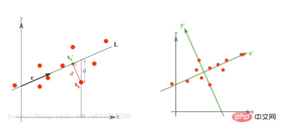 Minimal error theory dimensionality reduction principle
The minimum error is the linear projection that minimizes the average projection cost. In this process, we need to find parameters such as the squared error evaluation function J0(x0).
- Principal Component Analysis (PCA) code implementation
The code for the PCA algorithm is as follows:
from __future__ import print_function
from sklearn import datasets
import matplotlib.pyplot as plt
import matplotlib.cm as cmx
import matplotlib.colors as colors
import numpy as np
%matplotlib inline

def shuffle_data(X, y, seed=None):
 if seed:
 np.random.seed(seed)

 idx = np.arange(X.shape[0])
 np.random.shuffle(idx)

 return X[idx], y[idx]

# 正规化数据集 X
def normalize(X, axis=-1, p=2):
 lp_norm = np.atleast_1d(np.linalg.norm(X, p, axis))
 lp_norm[lp_norm == 0] = 1
 return X / np.expand_dims(lp_norm, axis)

# 标准化数据集 X
def standardize(X):
 X_std = np.zeros(X.shape)
 mean = X.mean(axis=0)
 std = X.std(axis=0)

 # 做除法运算时请永远记住分母不能等于 0 的情形
 # X_std = (X - X.mean(axis=0)) / X.std(axis=0)
 for col in range(np.shape(X)[1]):
 if std[col]:
 X_std[:, col] = (X_std[:, col] - mean[col]) / std[col]
 return X_std

# 划分数据集为训练集和测试集
def train_test_split(X, y, test_size=0.2, shuffle=True, seed=None):
 if shuffle:
 X, y = shuffle_data(X, y, seed)
 n_train_samples = int(X.shape[0] * (1-test_size))
 x_train, x_test = X[:n_train_samples], X[n_train_samples:]
 y_train, y_test = y[:n_train_samples], y[n_train_samples:]

 return x_train, x_test, y_train, y_test

# 计算矩阵 X 的协方差矩阵
def calculate_covariance_matrix(X, Y=np.empty((0,0))):
 if not Y.any():
Y = X
 n_samples = np.shape(X)[0]
 covariance_matrix = (1 / (n_samples-1)) * (X - X.mean(axis=0)).T.dot(Y - Y.mean(axis=0))
 return np.array(covariance_matrix, dtype=float)

# 计算数据集 X 每列的方差
def calculate_variance(X):
 n_samples = np.shape(X)[0]
 variance = (1 / n_samples) * np.diag((X - X.mean(axis=0)).T.dot(X - X.mean(axis=0)))
 return variance

# 计算数据集 X 每列的标准差
def calculate_std_dev(X):
 std_dev = np.sqrt(calculate_variance(X))
 return std_dev

# 计算相关系数矩阵
def calculate_correlation_matrix(X, Y=np.empty([0])):
 # 先计算协方差矩阵
 covariance_matrix = calculate_covariance_matrix(X, Y)
 # 计算 X, Y 的标准差
 std_dev_X = np.expand_dims(calculate_std_dev(X), 1)
 std_dev_y = np.expand_dims(calculate_std_dev(Y), 1)
 correlation_matrix = np.divide(covariance_matrix, std_dev_X.dot(std_dev_y.T))

 return np.array(correlation_matrix, dtype=float)

class PCA():
 """
 主成份分析算法 PCA,非监督学习算法.
 """
 def __init__(self):
 self.eigen_values = None
 self.eigen_vectors = None
 self.k = 2

 def transform(self, X):
 """
 将原始数据集 X 通过 PCA 进行降维
 """
 covariance = calculate_covariance_matrix(X)

 # 求解特征值和特征向量
 self.eigen_values, self.eigen_vectors = np.linalg.eig(covariance)

 # 将特征值从大到小进行排序,注意特征向量是按列排的,即 self.eigen_vectors 第 k 列是 self.eigen_values 中第 k 个特征值对应的特征向量
 idx = self.eigen_values.argsort()[::-1]
 eigenvalues = self.eigen_values[idx][:self.k]
 eigenvectors = self.eigen_vectors[:, idx][:, :self.k]

 # 将原始数据集 X 映射到低维空间
 X_transformed = X.dot(eigenvectors)

 return X_transformed

def main():
 # Load the dataset
 data = datasets.load_iris()
 X = data.data
 y = data.target

 # 将数据集 X 映射到低维空间
 X_trans = PCA().transform(X)

 x1 = X_trans[:, 0]
 x2 = X_trans[:, 1]

 cmap = plt.get_cmap('viridis')
 colors = [cmap(i) for i in np.linspace(0, 1, len(np.unique(y)))]

 class_distr = []
 # Plot the different class distributions
 for i, l in enumerate(np.unique(y)):
 _x1 = x1[y == l]
 _x2 = x2[y == l]
 _y = y[y == l]
 class_distr.append(plt.scatter(_x1, _x2, color=colors[i]))

 # Add a legend
 plt.legend(class_distr, y, loc=1)

 # Axis labels
 plt.xlabel('Principal Component 1')
 plt.ylabel('Principal Component 2')
 plt.show()

if __name__ == "__main__":
 main()
Finally , we will get the dimensionality reduction results as follows. Among them, if you get that when the number of features (D) is much larger than the number of samples (N), you can use a little trick to implement the complexity conversion of the PCA algorithm.
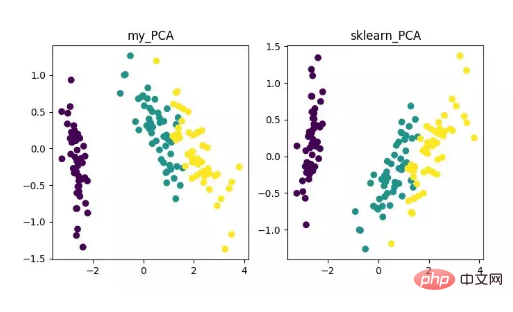
PCA dimensionality reduction algorithm display
Of course, although this algorithm is classic and commonly used, its shortcomings are also very obvious. It can remove linear correlation very well, but when faced with high-order correlation, the effect is poor; at the same time, the premise of PCA implementation is to assume that the main features of the data are distributed in the orthogonal direction, so for non-orthogonal directions There are several directions with large variances, and the effect of PCA will be greatly reduced.
Other dimensionality reduction algorithms and code addresses
- KPCA(kernel PCA)
KPCA is the product of the combination of kernel technology and PCA. It is mainly related to PCA The difference is that the kernel function is used when calculating the covariance matrix, which is the covariance matrix after mapping by the kernel function.
The introduction of kernel function can solve the nonlinear data mapping problem very well. kPCA can map nonlinear data to a high-dimensional space, where standard PCA is used to map it to another low-dimensional space.
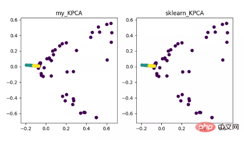
KPCA dimensionality reduction algorithm display
Code address:
https://github.com/heucoder/dimensionality_reduction_alo_codes/blob/master /codes/PCA/KPCA.py
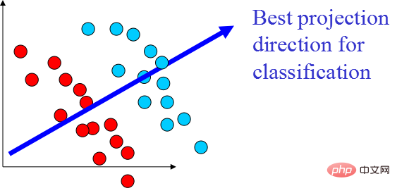
- LDA(Linear Discriminant Analysis)
LDA is a technology that can be used as a feature extraction, and its goal is to maximize the class Inter-class differences, minimizing the directional projection of intra-class differences, in order to facilitate tasks such as classification, that is, to effectively separate samples of different classes. LDA can improve the computational efficiency in the data analysis process, and can reduce overfitting caused by the disaster of dimensionality for models that cannot be regularized.
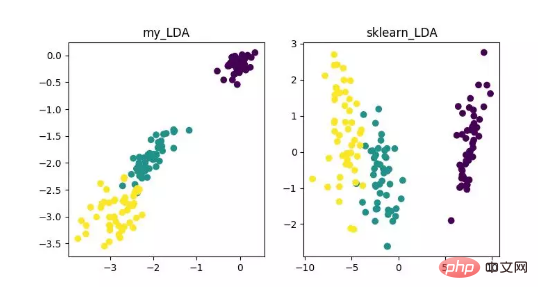
LDA dimensionality reduction algorithm display
Code address:
https://github.com/heucoder/dimensionality_reduction_alo_codes/tree/master /codes/LDA
- MDS(multidimensional scaling)
MDS is multidimensional scaling analysis. It is a method that expresses the perception and preferences of research objects through intuitive spatial diagrams. Traditional dimensionality reduction methods. This method calculates the distance between any two sample points so that the relative distance can be maintained after projection into a low-dimensional space to achieve projection.
Since MDS in sklearn adopts iterative optimization method, both iterative and non-iterative methods are implemented below.
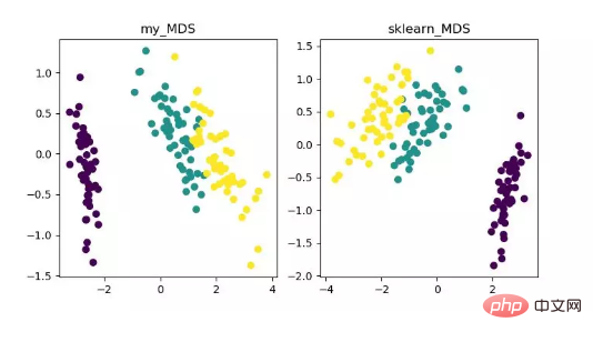
MDS dimensionality reduction algorithm display
Code address:
https://github.com/heucoder/dimensionality_reduction_alo_codes/tree/master /codes/MDS
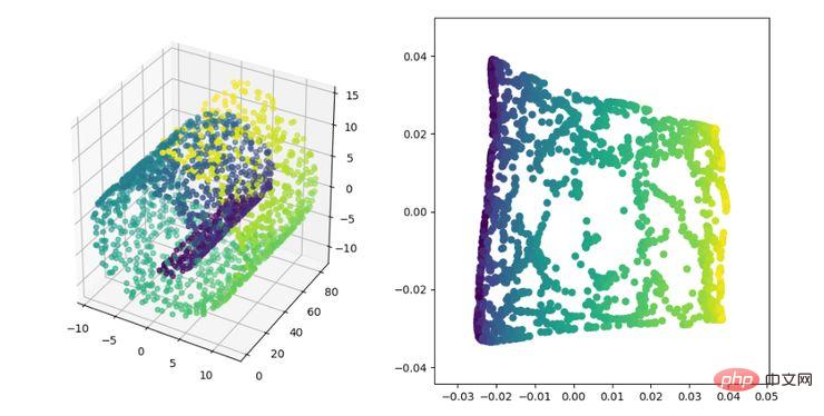
- ISOMAP
Isomap is an equimetric mapping algorithm. This algorithm can well solve the shortcomings of the MDS algorithm on non-linear structured data sets.
The MDS algorithm keeps the distance between samples after dimensionality reduction unchanged, while the Isomap algorithm introduces a neighborhood graph. The samples are only connected to their adjacent samples, calculate the distance between neighboring points, and then add them here On the basis of dimensionality reduction and distance preservation.
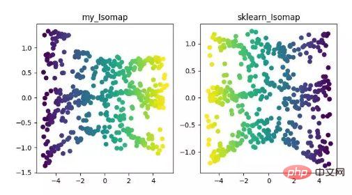
ISOMAP dimensionality reduction algorithm display
Code address:
https://github.com/heucoder/dimensionality_reduction_alo_codes/tree/master /codes/ISOMAP
LLE(locally linear embedding)LLE is the local linear embedding algorithm, which is a nonlinear dimensionality reduction algorithm. The core idea of this algorithm is that each point can be approximately reconstructed by a linear combination of multiple adjacent points, and then the high-dimensional data is projected into a low-dimensional space so that it maintains the local linear reconstruction between the data points. relationship, that is, have the same reconstruction coefficient. When dealing with so-called manifold dimensionality reduction, the effect is much better than PCA.
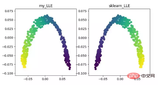
LLE dimensionality reduction algorithm display
Code address:
https://github.com/heucoder/dimensionality_reduction_alo_codes/tree/master/codes/LLE
- t-SNE
t-SNE is also a nonlinear dimensionality reduction algorithm, which is very suitable for reducing high-dimensional data to 2 or 3 dimensions for visualization. It is an unsupervised machine learning algorithm that reconstructs the data trend in low latitude (two or three dimensions) based on the original trend of the data.
The following result display refers to the source code, and can also be implemented with tensorflow (no need to manually update parameters).
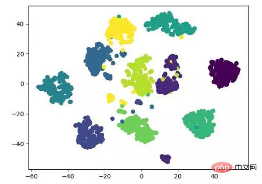
t-SNE dimensionality reduction algorithm display
Code address:
https://github.com/heucoder/dimensionality_reduction_alo_codes/tree /master/codes/T-SNE
- LE(Laplacian Eigenmaps)
LE is the Laplacian Eigenmap, which is somewhat similar to the LLE algorithm and is also based on local From the perspective of constructing the relationship between data. Its intuitive idea is to hope that points that are related to each other (points connected in the graph) are as close as possible in the dimensionally reduced space; in this way, a solution that can reflect the geometric structure of the manifold can be obtained.
LE dimensionality reduction algorithm display
Code address:
https://github.com/heucoder/dimensionality_reduction_alo_codes/tree/master /codes/LE
- LPP (Locality Preserving Projections)
LPP is the locality preserving projection algorithm. Its idea is similar to Laplacian feature mapping. The core idea is to pass It is best to maintain the neighbor structure information of a data set to construct projection mapping, but LPP is different from LE in directly obtaining the projection result, which requires solving the projection matrix.
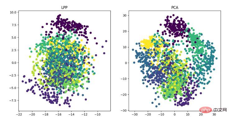
LPP dimensionality reduction algorithm display
Code address:
https://github.com/heucoder/dimensionality_reduction_alo_codes/tree/master /codes/LPP
- *About the author of the "dimensionality_reduction_alo_codes" project
Heucoder is currently a master's student in computer technology at Harbin Institute of Technology, mainly active in the Internet field, Zhihu The nickname is "Super Love Learning", and its github homepage address is: https://github.com/heucoder.
Github project address:
https://github.com/heucoder/dimensionality_reduction_alo_codes
The above is the detailed content of Python implements 12 dimensionality reduction algorithms. For more information, please follow other related articles on the PHP Chinese website!