


As far as machine learning is concerned, audio itself is a complete field with a wide range of applications, including speech recognition, music classification, sound event detection, etc. Audio classification has traditionally used methods such as spectrogram analysis and hidden Markov models, which have proven effective but also have their limitations. Recently VIT has emerged as a promising alternative for audio tasks, with OpenAI’s Whisper being a good example.

Dataset Introduction
GTZAN dataset is the most commonly used public dataset in music genre recognition (MGR) research. The files were collected in 2000-2001 from a variety of sources, including personal CDs, radios, microphone recordings, and represent sounds under a variety of recording conditions.

This data set consists of subfolders, each subfolder is of a type.

Loading data set
We will load each .wav file and generate the corresponding Mel spectrum through the librosa library.
The mel spectrogram is a visual representation of the spectral content of a sound signal. Its vertical axis represents frequency on the mel scale and the horizontal axis represents time. It is a commonly used representation in audio signal processing, especially in the field of music information retrieval.
Mel scale (English: mel scale) is a scale that takes into account human pitch perception. Because humans do not perceive linear ranges of frequencies, this means we are better at detecting differences at low frequencies than at high frequencies. For example, we can easily tell the difference between 500 Hz and 1000 Hz, but we have a harder time telling the difference between 10,000 Hz and 10,500 Hz, even if the distance between them is the same. So the Mel scale solves this problem, if the differences in the Mel scale are the same, that means the pitch differences perceived by humans will be the same.
def wav2melspec(fp):
 y, sr = librosa.load(fp)
 S = librosa.feature.melspectrogram(y=y, sr=sr, n_mels=128)
 log_S = librosa.amplitude_to_db(S, ref=np.max)
 img = librosa.display.specshow(log_S, sr=sr, x_axis='time', y_axis='mel')
 # get current figure without white border
 img = plt.gcf()
 img.gca().xaxis.set_major_locator(plt.NullLocator())
 img.gca().yaxis.set_major_locator(plt.NullLocator())
 img.subplots_adjust(top = 1, bottom = 0, right = 1, left = 0,
 hspace = 0, wspace = 0)
 img.gca().xaxis.set_major_locator(plt.NullLocator())
 img.gca().yaxis.set_major_locator(plt.NullLocator())
 # to pil image
 img.canvas.draw()
 img = Image.frombytes('RGB', img.canvas.get_width_height(), img.canvas.tostring_rgb())
 return img
The above function will produce a simple mel spectrogram:

Now we load the dataset from the folder and apply the transformation to the image.
class AudioDataset(Dataset):
 def __init__(self, root, transform=None):
 self.root = root
 self.transform = transform
 self.classes = sorted(os.listdir(root))
 self.class_to_idx = {c: i for i, c in enumerate(self.classes)}
 self.samples = []
 for c in self.classes:
 for fp in os.listdir(os.path.join(root, c)):
 self.samples.append((os.path.join(root, c, fp), self.class_to_idx[c]))

 def __len__(self):
 return len(self.samples)

 def __getitem__(self, idx):
 fp, target = self.samples[idx]
 img = Image.open(fp)
 if self.transform:
 img = self.transform(img)
 return img, target

 train_dataset = AudioDataset(root, transform=transforms.Compose([
 transforms.Resize((480, 480)),
 transforms.ToTensor(),
 transforms.Normalize((0.5, 0.5, 0.5), (0.5, 0.5, 0.5))
 ]))
ViT model
We will use ViT as our model: Vision Transformer first introduced an image equal to 16x16 words in the paper, and successfully demonstrated that this method does not Relying on any CNN, a pure Transformer applied directly to the sequence of image patches can perform image classification tasks well.
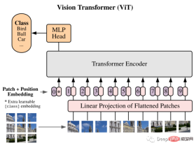
Split the image into Patches, and use the linear embedding sequence of these Patches as the input of the Transformer. Patches are treated in the same way as tokens (words) in NLP applications.
Due to the lack of inductive bias (such as locality) inherent in CNN, Transformer cannot generalize well when the amount of training data is insufficient. But when trained on large datasets, it does meet or beat the state-of-the-art on multiple image recognition benchmarks.
The implemented structure is as follows:
class ViT(nn.Sequential):
 def __init__(self,
 in_channels: int = 3,
 patch_size: int = 16,
 emb_size: int = 768,
 img_size: int = 356,
 depth: int = 12,
 n_classes: int = 1000,
 **kwargs):
 super().__init__(
 PatchEmbedding(in_channels, patch_size, emb_size, img_size),
 TransformerEncoder(depth, emb_size=emb_size, **kwargs),
 ClassificationHead(emb_size, n_classes)
Training
The training cycle is also a traditional training process:
vit = ViT(
 n_classes = len(train_dataset.classes)
 )

 vit.to(device)

 # train
 train_loader = DataLoader(train_dataset, batch_size=32, shuffle=True)
 optimizer = optim.Adam(vit.parameters(), lr=1e-3)
 scheduler = ReduceLROnPlateau(optimizer, 'max', factor=0.3, patience=3, verbose=True)
 criterion = nn.CrossEntropyLoss()
 num_epochs = 30

 for epoch in range(num_epochs):
 print('Epoch {}/{}'.format(epoch, num_epochs - 1))
 print('-' * 10)

 vit.train()

 running_loss = 0.0
 running_corrects = 0

 for inputs, labels in tqdm.tqdm(train_loader):
 inputs = inputs.to(device)
 labels = labels.to(device)

 optimizer.zero_grad()

 with torch.set_grad_enabled(True):
 outputs = vit(inputs)
 loss = criterion(outputs, labels)

 _, preds = torch.max(outputs, 1)
 loss.backward()
 optimizer.step()

 running_loss += loss.item() * inputs.size(0)
 running_corrects += torch.sum(preds == labels.data)

 epoch_loss = running_loss / len(train_dataset)
 epoch_acc = running_corrects.double() / len(train_dataset)
 scheduler.step(epoch_acc)

 print('Loss: {:.4f} Acc: {:.4f}'.format(epoch_loss, epoch_acc))
Summary
Usage PyTorch trained this custom implementation of the Vision Transformer architecture from scratch. Because the dataset is very small (only 100 samples per class), this affects the performance of the model, and only an accuracy of 0.71 was obtained.
This is just a simple demonstration. If you need to improve the model performance, you can use a larger data set, or slightly adjust the various hyperparameters of the architecture!
The vit code used here comes from:
https://medium.com/artificialis/vit-visiontransformer-a-pytorch-implementation-8d6a1033bdc5
The above is the detailed content of From video to audio: audio classification using VIT. For more information, please follow other related articles on the PHP Chinese website!

 2023年机器学习的十大概念和技术Apr 04, 2023 pm 12:30 PM
机器学习是一个不断发展的学科,一直在创造新的想法和技术。本文罗列了2023年机器学习的十大概念和技术。 本文罗列了2023年机器学习的十大概念和技术。2023年机器学习的十大概念和技术是一个教计算机从数据中学习的过程,无需明确的编程。机器学习是一个不断发展的学科,一直在创造新的想法和技术。为了保持领先,数据科学家应该关注其中一些网站,以跟上最新的发展。这将有助于了解机器学习中的技术如何在实践中使用,并为自己的业务或工作领域中的可能应用提供想法。2023年机器学习的十大概念和技术:1. 深度神经网
 人工智能自动获取知识和技能,实现自我完善的过程是什么Aug 24, 2022 am 11:57 AM
实现自我完善的过程是“机器学习”。机器学习是人工智能核心,是使计算机具有智能的根本途径;它使计算机能模拟人的学习行为,自动地通过学习来获取知识和技能,不断改善性能,实现自我完善。机器学习主要研究三方面问题:1、学习机理,人类获取知识、技能和抽象概念的天赋能力;2、学习方法,对生物学习机理进行简化的基础上,用计算的方法进行再现;3、学习系统,能够在一定程度上实现机器学习的系统。
 超参数优化比较之网格搜索、随机搜索和贝叶斯优化Apr 04, 2023 pm 12:05 PM
本文将详细介绍用来提高机器学习效果的最常见的超参数优化方法。 译者 | 朱先忠审校 | 孙淑娟简介通常,在尝试改进机器学习模型时,人们首先想到的解决方案是添加更多的训练数据。额外的数据通常是有帮助(在某些情况下除外)的,但生成高质量的数据可能非常昂贵。通过使用现有数据获得最佳模型性能,超参数优化可以节省我们的时间和资源。顾名思义,超参数优化是为机器学习模型确定最佳超参数组合以满足优化函数(即,给定研究中的数据集,最大化模型的性能)的过程。换句话说,每个模型都会提供多个有关选项的调整“按钮
 得益于OpenAI技术,微软必应的搜索流量超过谷歌Mar 31, 2023 pm 10:38 PM
截至3月20日的数据显示,自微软2月7日推出其人工智能版本以来,必应搜索引擎的页面访问量增加了15.8%,而Alphabet旗下的谷歌搜索引擎则下降了近1%。 3月23日消息,外媒报道称,分析公司Similarweb的数据显示,在整合了OpenAI的技术后,微软旗下的必应在页面访问量方面实现了更多的增长。截至3月20日的数据显示,自微软2月7日推出其人工智能版本以来,必应搜索引擎的页面访问量增加了15.8%,而Alphabet旗下的谷歌搜索引擎则下降了近1%。这些数据是微软在与谷歌争夺生
 荣耀的人工智能助手叫什么名字Sep 06, 2022 pm 03:31 PM
荣耀的人工智能助手叫“YOYO”,也即悠悠;YOYO除了能够实现语音操控等基本功能之外,还拥有智慧视觉、智慧识屏、情景智能、智慧搜索等功能,可以在系统设置页面中的智慧助手里进行相关的设置。
 人工智能在教育领域的应用主要有哪些Dec 14, 2020 pm 05:08 PM
人工智能在教育领域的应用主要有个性化学习、虚拟导师、教育机器人和场景式教育。人工智能在教育领域的应用目前还处于早期探索阶段,但是潜力却是巨大的。
 30行Python代码就可以调用ChatGPT API总结论文的主要内容Apr 04, 2023 pm 12:05 PM
阅读论文可以说是我们的日常工作之一,论文的数量太多,我们如何快速阅读归纳呢?自从ChatGPT出现以后,有很多阅读论文的服务可以使用。其实使用ChatGPT API非常简单,我们只用30行python代码就可以在本地搭建一个自己的应用。 阅读论文可以说是我们的日常工作之一,论文的数量太多,我们如何快速阅读归纳呢?自从ChatGPT出现以后,有很多阅读论文的服务可以使用。其实使用ChatGPT API非常简单,我们只用30行python代码就可以在本地搭建一个自己的应用。使用 Python 和 C
 人工智能在生活中的应用有哪些Jul 20, 2022 pm 04:47 PM
人工智能在生活中的应用有:1、虚拟个人助理,使用者可通过声控、文字输入的方式,来完成一些日常生活的小事;2、语音评测,利用云计算技术,将自动口语评测服务放在云端,并开放API接口供客户远程使用;3、无人汽车,主要依靠车内的以计算机系统为主的智能驾驶仪来实现无人驾驶的目标;4、天气预测,通过手机GPRS系统,定位到用户所处的位置,在利用算法,对覆盖全国的雷达图进行数据分析并预测。


Hot AI Tools

Undresser.AI Undress
AI-powered app for creating realistic nude photos

AI Clothes Remover
Online AI tool for removing clothes from photos.

Undress AI Tool
Undress images for free

Clothoff.io
AI clothes remover

AI Hentai Generator
Generate AI Hentai for free.

Hot Article
Hot Tools

MantisBT
Mantis is an easy-to-deploy web-based defect tracking tool designed to aid in product defect tracking. It requires PHP, MySQL and a web server. Check out our demo and hosting services.

mPDF
mPDF is a PHP library that can generate PDF files from UTF-8 encoded HTML. The original author, Ian Back, wrote mPDF to output PDF files "on the fly" from his website and handle different languages. It is slower than original scripts like HTML2FPDF and produces larger files when using Unicode fonts, but supports CSS styles etc. and has a lot of enhancements. Supports almost all languages, including RTL (Arabic and Hebrew) and CJK (Chinese, Japanese and Korean). Supports nested block-level elements (such as P, DIV),

Zend Studio 13.0.1
Powerful PHP integrated development environment

Dreamweaver CS6
Visual web development tools

Safe Exam Browser
Safe Exam Browser is a secure browser environment for taking online exams securely. This software turns any computer into a secure workstation. It controls access to any utility and prevents students from using unauthorized resources.

