 Technology peripherals
 AI
AI Numerical distance based on machine learning: the distance between points in space
Numerical distance based on machine learning: the distance between points in space
This article is reproduced from the WeChat public account "Living in the Information Age". The author lives in the information age. To reprint this article, please contact the Living in the Information Age public account.
In machine learning, a basic concept is how to judge the difference between two samples, so as to be able to evaluate the similarity and category information between the two samples. The measure to judge this similarity is the distance between two samples in the feature space.
There are many measurement methods based on different data characteristics. Generally speaking, for two data samples x, y, define a function d(x, y). If it is defined as the distance between the two samples, then d(x, y) needs to satisfy the following basic properties :
- Non-negativity: d(x,y)>=0
- Identity: d(x,y)=0 ⇔ x=y
- Symmetry: d (x, y) = d (y, x)
- Triangle inequality: d (x, y)
Generally speaking, common distance measures include: distance between points in space, distance between strings, similarity of sets, and distance between variable/concept distributions.
Today we will first introduce the distance between the most commonly used points in space.
The distance between points in space includes the following types:
1. Euclidean Distance
There is no doubt that, Euclidean distance is the distance that people are most familiar with. It is the straight-line distance between two points. Students who have studied junior high school mathematics all know how to calculate the distance between two points in two-dimensional space in the Cartesian coordinate system
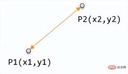
The calculation formula is:


2. Manhattan Distance
Manhattan distance is also called taxi distance. Its concept comes from the many horizontal and vertical blocks in Manhattan, New York. , in this kind of neighborhood, if a taxi driver wants to walk from one point to another, it is useless to calculate the straight-line distance, because the taxi cannot fly over the buildings. Therefore, this distance is usually calculated by subtracting and adding the east-west and north-south distances of two points respectively. This is the actual distance that the taxi has to travel.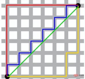

3. Chebyshev Distance (Chebyshev Distance)
Chebyshev distance is defined as the maximum value of the difference in coordinate values between two points.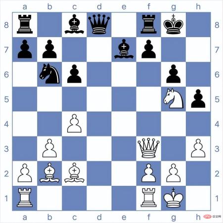
The Min distance itself is not a special distance, but a formula that combines multiple distances (Manhattan distance, Euclidean distance, Chebyshev distance).
It is defined as, for two n-dimensional variables, the Min's distance is:

When p=1, you can see
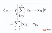
At this time is the Manhattan distance.
When p=2, you can see that
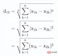
is the Euclidean distance.
When p=∞, you can see that
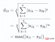
This is the Chebyshev distance.
5. Standardized Euclidean Distance
Euclidean distance can measure the straight-line distance between two points, but in some cases In some cases, it may be affected by different units. For example, if there is a height difference of 5 mm and a weight difference of 5 kg at the same time, the perception may be completely different. If we want to cluster three models, their respective attributes are as follows:
A: 65000000 mg (ie 65 kg), 1.74 m
B: 60000000 mg (ie 60 kg) , 1.70 meters
C: 65,000,000 mg (i.e. 65 kg), 1.40 meters
According to our normal understanding, A and B are models with better figures and should be classified into the same category. However, when actually calculating in the above units, it is found that the difference between A and B is greater than the difference between A and C. The reason is that the different measurement units of attributes lead to excessive numerical differences. If the same data is changed to another unit.
A: 65kg, 174cm
B: 60kg, 170cm
C: 65kg, 140cm
Then we will get The result that comes to mind is that A and B are classified into the same category. Therefore, in order to avoid such differences due to different measurement units, we need to introduce standardized Euclidean distance. In this distance calculation, each component is normalized to an interval with equal mean and variance.
Assume that the mean (mean) of the sample set X is m and the standard deviation (standard deviation) is s, then the "standardized variable" of X is expressed as:


6. Lance and Williams Distance
Lance distance is also called Canberra distance, 
7. Mahalanobis Distance
After standardizing the values, will there be no problems? maybe. For example, in a one-dimensional example, if there are two classes, one class has a mean of 0 and a variance of 0.1, and the other class has a mean of 5 and a variance of 5. So if a point with a value of 2 should belong to which category? We intuitively think that it must be the second category, because the first category is obviously unlikely to reach 2 numerically. But in fact, if calculated from the distance, the number 2 must belong to the first category.
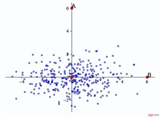
So, in a dimension with small variance, a small difference may become an outlier. For example, in the figure below, A and B are at the same distance from the origin, but since the entire sample is distributed along the horizontal axis, point B is more likely to be a point in the sample, while point A is more likely to be an outlier. .
Problems may also occur when the dimensions are not independently and identically distributed. For example, point A and point B in the figure below are The origins are equally distant, but the main distribution is similar to f(x)=x, so A is more like an outlier.
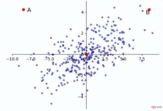
Therefore, we can see that in this case, the standardized Euclidean distance will also have problems, so we need to introduce Mahalanobis distance.
The Mahalanobis distance rotates the variables according to the principal components to make the dimensions independent of each other, and then standardizes them to make the dimensions equally distributed. The principal component is the direction of the eigenvector, so you only need to rotate according to the direction of the eigenvector, and then scale the eigenvalue times. For example, after the above image is transformed, the following result will be obtained:
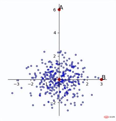
It can be seen that the outliers have been successfully separated.
The Mahalanobis distance was proposed by the Indian mathematician Mahalanobis and represents the covariance distance of the data. It is an efficient method to calculate the similarity of two unknown sample sets.
For a multivariate vector with mean

and covariance matrix Σ

, its Mahalanobis distance (the Mahalanobis distance of a single data point) is:

For The degree of difference between two random variables X and Y that obey the same distribution and whose covariance matrix is Σ. The Mahalanobis distance between data points x and y is:

If the covariance matrix is the identity matrix, then the Mahalanobis distance is simplified to the Euclidean distance. If the covariance matrix is a diagonal matrix, then the Mahalanobis distance becomes the standardized Euclidean distance.
8. Cosine Distance
As the name suggests, cosine distance comes from the cosine of the angle in geometry, which can be used to measure the difference in the direction of two vectors. rather than distance or length. When the cosine value is 0, the two vectors are orthogonal and the included angle is 90 degrees. The smaller the angle is, the closer the cosine value is to 1 and the direction is more consistent.
In N-dimensional space, the cosine distance is:
It is worth pointing out that the cosine distance does not satisfy the triangle inequality.
9. Geodesic Distance
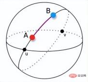
Geodesic distance originally refers to the shortest distance between the surfaces of spheres. When the feature space is a plane, the geodesic distance is the Euclidean distance. In non-Euclidean geometry, the shortest line between two points on the sphere is the great arc connecting the two points. The sides of triangles and polygons on the sphere are also composed of these great arcs.
10. Bray Curtis Distance
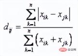
Bray Curtis distance is mainly used Botany, Ecology and Environmental Sciences, it can be used to calculate differences between samples. The formula is:
The above is the detailed content of Numerical distance based on machine learning: the distance between points in space. For more information, please follow other related articles on the PHP Chinese website!
 Let's Dance: Structured Movement To Fine-Tune Our Human Neural NetsApr 27, 2025 am 11:09 AM
Scientists have extensively studied human and simpler neural networks (like those in C. elegans) to understand their functionality. However, a crucial question arises: how do we adapt our own neural networks to work effectively alongside novel AI s
 New Google Leak Reveals Subscription Changes For Gemini AIApr 27, 2025 am 11:08 AM
Google's Gemini Advanced: New Subscription Tiers on the Horizon Currently, accessing Gemini Advanced requires a $19.99/month Google One AI Premium plan. However, an Android Authority report hints at upcoming changes. Code within the latest Google P
 How Data Analytics Acceleration Is Solving AI's Hidden BottleneckApr 27, 2025 am 11:07 AM
Despite the hype surrounding advanced AI capabilities, a significant challenge lurks within enterprise AI deployments: data processing bottlenecks. While CEOs celebrate AI advancements, engineers grapple with slow query times, overloaded pipelines, a
 MarkItDown MCP Can Convert Any Document into Markdowns!Apr 27, 2025 am 09:47 AM
Handling documents is no longer just about opening files in your AI projects, it’s about transforming chaos into clarity. Docs such as PDFs, PowerPoints, and Word flood our workflows in every shape and size. Retrieving structured
 How to Use Google ADK for Building Agents? - Analytics VidhyaApr 27, 2025 am 09:42 AM
Harness the power of Google's Agent Development Kit (ADK) to create intelligent agents with real-world capabilities! This tutorial guides you through building conversational agents using ADK, supporting various language models like Gemini and GPT. W
 Use of SLM over LLM for Effective Problem Solving - Analytics VidhyaApr 27, 2025 am 09:27 AM
summary: Small Language Model (SLM) is designed for efficiency. They are better than the Large Language Model (LLM) in resource-deficient, real-time and privacy-sensitive environments. Best for focus-based tasks, especially where domain specificity, controllability, and interpretability are more important than general knowledge or creativity. SLMs are not a replacement for LLMs, but they are ideal when precision, speed and cost-effectiveness are critical. Technology helps us achieve more with fewer resources. It has always been a promoter, not a driver. From the steam engine era to the Internet bubble era, the power of technology lies in the extent to which it helps us solve problems. Artificial intelligence (AI) and more recently generative AI are no exception
 How to Use Google Gemini Models for Computer Vision Tasks? - Analytics VidhyaApr 27, 2025 am 09:26 AM
Harness the Power of Google Gemini for Computer Vision: A Comprehensive Guide Google Gemini, a leading AI chatbot, extends its capabilities beyond conversation to encompass powerful computer vision functionalities. This guide details how to utilize
 Gemini 2.0 Flash vs o4-mini: Can Google Do Better Than OpenAI?Apr 27, 2025 am 09:20 AM
The AI landscape of 2025 is electrifying with the arrival of Google's Gemini 2.0 Flash and OpenAI's o4-mini. These cutting-edge models, launched weeks apart, boast comparable advanced features and impressive benchmark scores. This in-depth compariso


Hot AI Tools

Undresser.AI Undress
AI-powered app for creating realistic nude photos

AI Clothes Remover
Online AI tool for removing clothes from photos.

Undress AI Tool
Undress images for free

Clothoff.io
AI clothes remover

Video Face Swap
Swap faces in any video effortlessly with our completely free AI face swap tool!

Hot Article

Hot Tools

SublimeText3 English version
Recommended: Win version, supports code prompts!

ZendStudio 13.5.1 Mac
Powerful PHP integrated development environment

Safe Exam Browser
Safe Exam Browser is a secure browser environment for taking online exams securely. This software turns any computer into a secure workstation. It controls access to any utility and prevents students from using unauthorized resources.

SublimeText3 Chinese version
Chinese version, very easy to use

EditPlus Chinese cracked version
Small size, syntax highlighting, does not support code prompt function


