Cool, Python realizes traffic data visualization!

1. Introduction to TransBigData

TransBigData handles common traffic spatio-temporal big data (such as taxi GPS data, shared bicycle data and bus GPS data, etc.) provides a quick and concise method. TransBigData provides a variety of processing methods for each stage of traffic spatio-temporal big data analysis. The code is concise, efficient, flexible and easy to use. Complex data tasks can be implemented with concise code.

Currently, TransBigData mainly provides the following methods:

• Data preprocessing: Provides methods for quickly calculating basic information such as data volume, time period, sampling interval, etc. for data sets, and also targets multiple data sets. This kind of data noise provides corresponding cleaning methods.
• Data rasterization: Provides a method system for generating and matching multiple types of geographical rasters (rectangular, triangular, hexagonal and geohash rasters) within the study area, which can be quickly vectorized The algorithm maps spatial point data onto a geographic raster.
• Data visualization: Based on the visualization package keplergl, data can be displayed interactively and visually on Jupyter Notebook with simple code.
• Trajectory processing: Generate trajectory line types from trajectory data GPS points, densify and sparse trajectory points, etc.
• Map base map, coordinate conversion and calculation: Load and display the coordinate conversion between the map base map and various special coordinate systems.
• Specific processing methods: Provide corresponding processing methods for various types of specific data, such as extracting order starting and ending points from taxi GPS data, identifying residence and work place from mobile phone signaling data, and subway network GIS data Build network topology and calculate shortest paths, etc.

TransBigData can be installed through pip or conda. Run the following code in the command prompt to install:

pip install -U transbigdata

After the installation is complete, run the following code in Python to import TransBigData Bag.

import transbigdata as tbd

2. Data preprocessing

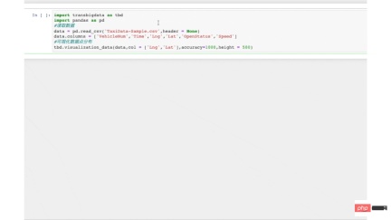
TransBigData can be seamlessly connected with Pandas and GeoPandas packages commonly used in data processing. First, we introduce the Pandas package and read the taxi GPS data:

import pandas as pd
# 读取数据
data = pd.read_csv('TaxiData-Sample.csv',header = None)
data.columns = ['VehicleNum','time','lon','lat','OpenStatus','Speed']
data.head()

The results are shown in Figure 2:

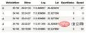
▲Figure 2 Taxi GPS data

Then, introduce the GeoPandas package, read the regional information of the research scope and display:

import geopandas as gpd
# 读取研究范围区域信息
sz = gpd.read_file(r'sz/sz.shp')
sz.plot()

The results are shown in Figure 3:

▲Figure 3 Regional information of the research scope

The TransBigData package integrates some common preprocessing methods for traffic spatiotemporal data. Among them, the tbd.clean_outofshape method inputs data and research scope area information, and can eliminate data outside the research scope. The tbd.clean_taxi_status method can eliminate records of instantaneous changes in passenger status in taxi GPS data. When using the preprocessing method, you need to pass in the column names corresponding to the important information columns in the data table. The code is as follows:

# 数据预处理
#剔除研究范围外的数据，计算原理是在方法中先栅格化后栅格匹配研究范围后实现对应。因此这里需要同时定义栅格大小，越小则精度越高
data = tbd.clean_outofshape(data, sz, col=['lon', 'lat'], accuracy=500)
# 剔除出租车数据中载客状态瞬间变化的数据
data = tbd.clean_taxi_status(data, col=['VehicleNum', 'time', 'OpenStatus'])

After processing the above code, we have already converted the taxi GPS to Data outside the research scope and data on instantaneous changes in passenger status are eliminated from the data.

3. Data rasterization

The raster form (grids of the same size in geographical space) is the most basic way to express data distribution. After the GPS data is rasterized, each Data points contain information about the raster where they are located. When raster is used to express the distribution of data, the distribution it represents is close to the real situation.

TransBigData tool provides us with a complete, fast and convenient raster processing system. When using TransBigData for raster division, you first need to determine the rasterization parameters (which can be understood as defining a raster coordinate system). The parameters can help us quickly rasterize:

# 定义研究范围边界
bounds = [113.75, 22.4,114.62, 22.86]
# 通过边界获取栅格化参数
params = tbd.area_to_params(bounds,accuracy = 1000)
params

Output:

{'slon': 113.75,
'slat': 22.4,
'deltalon': 0.00974336289289822,
'deltalat': 0.008993210412845813,
'theta': 0,
'method': 'rect',
'gridsize': 1000}

The content of the rasterization parameter params output at this time stores the origin coordinates of the raster coordinate system (slon, slat), the longitude and latitude of a single raster. (deltalon, deltalat), the rotation angle of the grid (theta), the shape of the grid (method parameter, whose value can be square rect, triangle tri, and hexagon hexa) and the size of the grid (gridsize parameter, in meters ).

After obtaining the rasterization parameters, we can use the methods provided in TransBigData to perform operations such as raster matching and generation on GPS data.

The complete raster processing method system is shown in Figure 4:

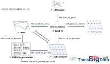
▲Figure 4 The raster processing system provided by TransBigData

Use the tbd.GPS_to_grid method to generate GPS points for each taxi. This method will generate number columns LONCOL and LATCOL, which together specify the grid:

# 将GPS数据对应至栅格，将生成的栅格编号列赋值到数据表上作为新的两列
data['LONCOL'],data['LATCOL']= tbd.GPS_to_grids(data['lon'],data['lat'],params)

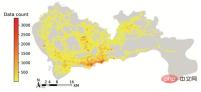
下一步，聚合集计每一栅格内的数据量，并为栅格生成地理几何图形，构建GeoDataFrame：

# 聚合集计栅格内数据量
grid_agg=data.groupby(['LONCOL','LATCOL'])['VehicleNum'].count().reset_index()
# 生成栅格的几何图形
grid_agg['geometry']=tbd.grid_to_polygon([grid_agg['LONCOL'],grid_agg['LATCOL']],params)
# 转换为GeoDataFrame
grid_agg=gpd.GeoDataFrame(grid_agg)
# 绘制栅格
grid_agg.plot(column = 'VehicleNum',cmap = 'autumn_r')

结果如图5所示：

▲图5 数据栅格化的结果

对于一个正式的数据可视化图来说，我们还需要添加底图、色条、指北针和比例尺。TransBigData也提供了相应的功能，代码如下：

import matplotlib.pyplot as plt
fig =plt.figure(1,(8,8),dpi=300)
ax =plt.subplot(111)
plt.sca(ax)
# 添加行政区划边界作为底图
sz.plot(ax=ax,edgecolor=(0,0,0,0),facecolor=(0,0,0,0.1),linewidths=0.5)
# 定义色条位置
cax = plt.axes([0.04, 0.33, 0.02, 0.3])
plt.title('Data count')
plt.sca(ax)
# 绘制数据
grid_agg.plot(column = 'VehicleNum',cmap = 'autumn_r',ax = ax,cax = cax,legend = True)
# 添加指北针和比例尺
tbd.plotscale(ax,bounds = bounds,textsize = 10,compasssize = 1,accuracy = 2000,rect = [0.06,0.03],zorder = 10)
plt.axis('off')
plt.xlim(bounds[0],bounds[2])
plt.ylim(bounds[1],bounds[3])
plt.show()

结果如图6所示：

▲图6 tbd包绘制的出租车GPS数据分布

4、订单起讫点OD提取与聚合集计

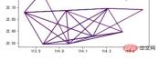
针对出租车GPS数据，TransBigData提供了直接从数据中提取出出租车订单起讫点（OD）信息的方法，代码如下：

# 从GPS数据提取OD
oddat=tbd.taxigps_to_od(data,col=['VehicleNum','time','Lng','Lat','OpenStatus'])
oddata

结果如图7所示：

▲图7 tbd包提取的出租车OD

TransBigData包提供的栅格化方法可以让我们快速地进行栅格化定义，只需要修改accuracy参数，即可快速定义不同大小粒度的栅格。我们重新定义一个2km*2km的栅格坐标系，将其参数传入tbd.odagg_grid方法对OD进行栅格化聚合集计并生成GeoDataFrame：

# 重新定义栅格，获取栅格化参数
params=tbd.area_to_params(bounds,accuracy = 2000)
# 栅格化OD并集计
od_gdf=tbd.odagg_grid(oddata,params)
od_gdf.plot(column = 'count')

结果如图8所示：

▲图8 tbd集计的栅格OD

添加地图底图，色条与比例尺指北针：

# 创建图框
import matplotlib.pyplot as plt
fig =plt.figure(1,(8,8),dpi=300)
ax =plt.subplot(111)
plt.sca(ax)
# 添加行政区划边界作为底图
sz.plot(ax=ax,edgecolor=(0,0,0,1),facecolor=(0,0,0,0),linewidths=0.5)
# 绘制colorbar
cax=plt.axes([0.05, 0.33, 0.02, 0.3])
plt.title('Data count')
plt.sca(ax)
# 绘制OD
od_gdf.plot(ax = ax,column = 'count',cmap = 'Blues_r',linewidth = 0.5,vmax = 10,cax = cax,legend = True)
# 添加比例尺和指北针
tbd.plotscale(ax,bounds=bounds,textsize=10,compasssize=1,accuracy=2000,rect = [0.06,0.03],zorder = 10)
plt.axis('off')
plt.xlim(bounds[0],bounds[2])
plt.ylim(bounds[1],bounds[3])
plt.show()

结果如图9所示：

▲ 图9 TransBigData绘制的栅格OD数据

同时，TransBigData包也提供了将OD直接聚合集计到区域间的方法：

# OD集计到区域
# 方法1：在不传入栅格化参数时，直接用经纬度匹配
od_gdf = tbd.odagg_shape(oddata,sz,round_accuracy=6)
# 方法2：传入栅格化参数时，程序会先栅格化后匹配以加快运算速度，数据量大时建议使用
od_gdf = tbd.odagg_shape(oddata,sz,params = params)
od_gdf.plot(column = 'count')

结果如图10所示：

▲图10 tbd集计的小区OD

加载地图底图并调整出图参数：

# 创建图框
import matplotlib.pyplot as plt
import plot_map
fig =plt.figure(1,(8,8),dpi=300)
ax =plt.subplot(111)
plt.sca(ax)
# 添加行政区划边界作为底图
sz.plot(ax = ax,edgecolor = (0,0,0,0),facecolor = (0,0,0,0.2),linewidths=0.5)
# 绘制colorbar
cax = plt.axes([0.05, 0.33, 0.02, 0.3])
plt.title('count')
plt.sca(ax)
# 绘制OD
od_gdf.plot(ax = ax,vmax = 100,column = 'count',cax = cax,cmap = 'autumn_r',linewidth = 1,legend = True)
# 添加比例尺和指北针
tbd.plotscale(ax,bounds = bounds,textsize = 10,compasssize = 1,accuracy = 2000,rect = [0.06,0.03],zorder = 10)
plt.axis('off')
plt.xlim(bounds[0],bounds[2])
plt.ylim(bounds[1],bounds[3])
plt.show()

结果如图11所示：

▲ 图11区域间OD可视化结果

5、交互可视化

在TransBigData中，我们可以对出租车数据使用简单的代码在jupyter notebook中快速进行交互可视化。这些可视化方法底层依托了keplergl包，可视化的结果不再是静态的图片，而是能够与鼠标响应交互的地图应用。

tbd.visualization_data方法可以实现数据分布的可视化，将数据传入该方法后，TransBigData会首先对数据点进行栅格集计，然后生成数据的栅格，并将数据量映射至颜色上。代码如下：

结果如图12所示：

# 可视化数据点分布
tbd.visualization_data(data,col = ['lon','lat'],accuracy=1000,height = 500)

▲ 图12数据分布的栅格可视化

对于出租车数据中所提取出的出行OD，也可使用tbd.visualization_od方法实现OD的弧线可视化。该方法也会对OD数据进行栅格聚合集计，生成OD弧线，并将不同大小的OD出行量映射至不同颜色。代码如下：

# 可视化数据点分布
tbd.visualization_od(oddata,accuracy=2000,height = 500)

结果如图13所示：

▲ 图13 OD分布的弧线可视化

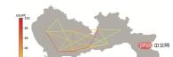
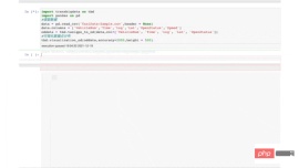
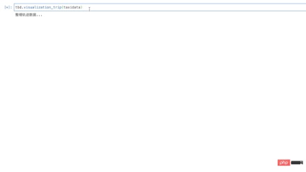
对个体级的连续追踪数据，tbd.visualization_trip方法可以将数据点处理为带有时间戳的轨迹信息并动态地展示，代码如下：

# 动态可视化轨迹
tbd.visualization_trip(data,col = ['lon','lat','VehicleNum','time'],height = 500)

结果图14所示。点击其中的播放键，可以看到出租车运行的动态轨迹效果。

The above is the detailed content of Cool, Python realizes traffic data visualization!. For more information, please follow other related articles on the PHP Chinese website!