How to make better use of data in causal inference?

Introduction: The title of this sharing is "How to make better use of data in causal inference?" ", which mainly introduces the team's recent work related to published papers on cause and effect. This report introduces how we can use more data to make causal inferences from two aspects. One is to use historical control data to explicitly mitigate confusion bias, and the other is causal inference under the fusion of multi-source data.
Full text table of contents:
- Causal inference background
- Correction Causal Tree GBCT
- Causal Data Fusion
- In Ant’s business applications
1. Causal inference background
Common machine learning prediction problems are generally Set in the same system, for example, independent and identical distribution is usually assumed, such as predicting the probability of lung cancer among smokers, picture classification and other prediction problems. The question of causation is concerned with the mechanism behind the data. Common questions such as "Does smoking cause lung cancer?" Similar questions are causation issues.
There are two very important types of data in the problem of causal effect estimation: one type is observation data, and the other type is experimental data generated by randomized controlled experiments. .
- Observation data is the data accumulated in our actual life or products. For example, the smoking data shows that some people like to smoke, while the observational data is related to smokers. In the end, some of the smokers will get cancer. The machine learning prediction problem is to estimate the conditional probability P (get lung cancer | smoking), that is, given the conditions of smoking, the probability of observing a smoker getting lung cancer. In the above observational data, the distribution of smoking is actually not random: everyone's preference for smoking is different, and it is also affected by the environment.
- #The best way to answer causal questions is to conduct a randomized controlled experiment. Experimental data are obtained through randomized controlled experiments. In a randomized controlled trial, assignment to treatment is random. Suppose you need to conduct an experiment to get the conclusion "whether smoking causes lung cancer." First, you need to find enough people, force half of them to smoke, and force the other half not to smoke, and observe the probability of lung cancer in the two groups. Although randomized controlled trials are not possible in some scenarios due to factors such as ethics and policies, randomized controlled trials can still be conducted in some fields, such as A/B testing in search promotion.
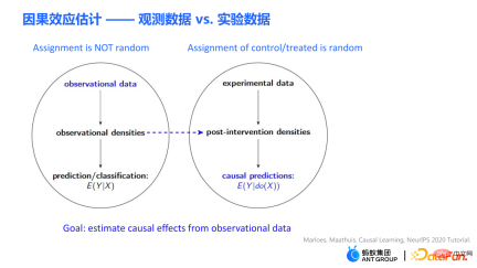
The causal estimation problem E(Y|do(X)) problem and the traditional prediction or classification problem The main difference between E(Y|X) is that the intervention symbol do proposed by Judy Pearl appears in the given condition. Intervene to force the X variable to a certain value. The estimation of causal effects in this report mainly refers to estimating causal effects from observational data.
#How to better utilize data in causal inference? This report will introduce such a topic using recent papers published by two teams as examples.
- The first job is how to make better use of historical comparison data. For example, if a marketing promotion event is held at a certain point in time, the time before this time point is called "pre-intervention", and the time after this time point is called "post-intervention". We hope to know the actual effect of intervention before we intervene, so as to assist us in making the next decision. Before the start of this marketing campaign, we have historical performance data of users. The first task is to introduce how to make good use of "pre-intervention" data to assist in data correction work to better evaluate the effect of intervention.
- #The second work mainly introduces how to better utilize multi-source heterogeneous data. Such problems are often involved in machine learning. Common problems include domain adaptation, transfer learning, etc. In today's report, we will consider the utilization of multi-source heterogeneous data from a causal perspective, that is, assuming that there are multiple data sources, how to better estimate the causal effect.
2. Corrective Cause and Effect Tree GBCT
1. Traditional Cause and Effect Tree
Tree algorithm mainly consists of two modules:
- Split criterion: Split a node into two child nodes according to the split criterion
- Parameter estimation: After the split is completed, for example, when the split is finally stopped, the causal effect of the new sample or group is predicted on the leaf node according to the parameter estimation method
Some traditional causal tree algorithms split based on the heterogeneity of causal effects. The basic idea is to hope that the causal effects of the left sub-node and the right sub-node after splitting will be significantly different, and the differences can be captured through splitting. Heterogeneity of causal effects in data distributions.
The splitting criterion of the traditional causal tree, such as:
- The splitting criterion of the uplift tree is to maximize the causal effect of the left and right child nodes Difference, the measure of difference uses distance measures such as Euclidean distance and KL divergence;
- ##causal tree splitting criterion can be intuitively explained as maximizing the square of the causal effect . It can be mathematically proven that this splitting criterion is equivalent to maximizing the variance of the causal effects of leaf nodes.
In the causal tree, the child nodes are obtained by splitting. Can we ensure that the distribution of the left child node and the right child node obtained by the split is homogeneous?
2. Correction Causal Tree GBCT
The traditional causal tree and uplift tree cannot guarantee the left-hand side after splitting. The distribution of child nodes and right child nodes is homogeneous. Therefore, the traditional estimates  # mentioned in the previous section are biased.

Our work focuses on estimating the average causal effect CATT over the experimental group (treatment group). CATT is defined as:

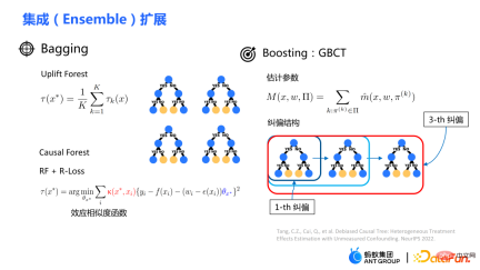
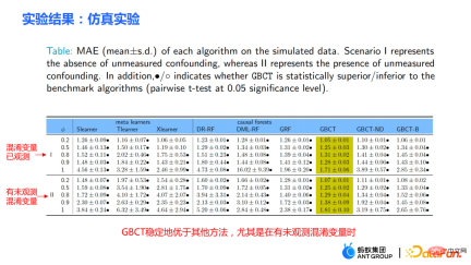
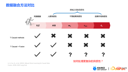
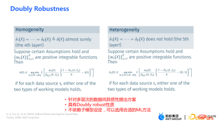
##Further, the traditional causal effect estimate can be split into two parts: Selection bias/confounding bias can be defined as: ##The intuitive meaning is the estimated value when treatment=0 in the experimental group, minus the estimated value when treatment=0 in the control group. In traditional causal trees, the above bias is not characterized, and selection bias may affect our estimates, resulting in the final estimate being biased. The intuitive meaning is: in the experimental group, use the model of the control group for estimation; In the control group, use the model of the experimental group for estimation; make the estimates of the two parts as close as possible, so that the distributions of the experimental group and the control group are as close to the same as possible. The use of confusion entropy is one of the main contributions of our work. The integration of traditional tree models includes methods such as bagging and boosting. The integration method used by uplift forest or causal forest is the bagging method. The integration of uplift forest is direct summation, while the integration of causal forest requires solving a loss function. Due to the explicit correction module designed in GBCT, GBCT supports integration using the boosting method. The basic idea is similar to boosting: after the first tree is corrected, the second tree is corrected, and the third tree is corrected... Two parts of experiments were done: ① Simulation experiment. Under simulation experiments containing ground truth, test whether the GBCT method can achieve the expected results. The data generation for the simulation experiment is divided into two parts (the first column Φ in the table represents selection bias. The larger the Φ value, the stronger the corresponding selection bias; the value in the table is MAE. The smaller the MAE value, the better the method) : ##②Real credit card limit increase data. A randomized controlled experiment was conducted, and biased data were constructed based on the randomized controlled experiment. Across different settings, the GBCT method consistently outperforms traditional methods, especially on biased data, performing significantly better than traditional methods. The second task is causal data fusion, that is, how to better Estimating causal effects. Main symbols: multiple data sources, Y is outcome, A is treatment, X is the association of concern Variables, Z are other covariates of each data source (domain) except X, S is the indicator of the domain used to indicate which domain it belongs to, and μ is the expected value of the potential outcome. Decompose the outcome into the following expression: ##target function δ is used to estimate the causal effect on each domain, In addition, nuisance functions include main effects, propensity scores, domain propensity scores, variances of effects, etc. Some traditional methods, such as meta learner, etc., assume that the data is of the same origin, that is, the distribution is consistent . Some traditional data fusion methods can handle the heterogeneity of populations across domains, but cannot explicitly capture the heterogeneity of intervention outcomes and causal effects across domains. Our work focuses on dealing with more complex heterogeneity across domains, including heterogeneity across domains in intervention outcomes and heterogeneity across domains in causal effects. The three modules are combined to get the final estimate. The three highlights of the WMDL algorithm are: In this work, we did not estimate the outcome of the experimental group and the outcome of the control group, and then make the difference to obtain the cause and effect. Instead of estimating the effect, we directly estimate the causal effect, that is, Direct Learning. The benefit of Direct Learning is that it can avoid higher frequency noise signals in the experimental and control groups. The left part assumes that the causal effects are the same among multiple domains, but the outcomes may be heterogeneous. ; The right part assumes that the causal effects between each domain are different, that is, between different domains, even if its covariates are the same, their causal effects are also different. The formula is derived based on the disassembly formula. Outcome Y minus main effect divided by treatment is estimated to be I(X), and the optimal solution obtained is δ(X). The numerator in This work has three advantages: ① Through different designs, it can not only handle the heterogeneity of intervention results, but also Deal with the heterogeneity between causal effects; ② It has the property of doubly robustness. The proof is given in the paper that as long as the estimate of either the domain's propensity score model or the main effect model is unbiased, the final estimate will be unbiased (the actual situation is a little more complicated, see the paper for details); #③ This work mainly designed the semi-parametric model framework. Each module of the model can use any machine learning model, and the entire model can even be designed into a neural network to achieve end-to-end learning. Weighting’s module is derived from the efficiency bound theory in statistics. It mainly contains two aspects of information: ① ② Through the design of the propensity score function on the denominator, the overlapping samples in the experimental group and the control group are given a comparative weight. Large weight; #③ Use V to characterize the noise in the data. Since the noise is in the denominator, samples with less noise will get larger weights. By cleverly combining the above three parts, the distribution differences between different domains and the performance of different causal information can be mapped into a unified domain . Regardless of homogeneous causal effects or heterogeneous causal effects, WMDL (Weighted Multi-domain Direct Learning ) methods have better results. The picture on the right shows an ablation experiment on the weighting module. The experiment shows the effectiveness of the weighting module. In summary, the WMDL method consistently performs better than other methods, and the estimated variance is relatively small. In financial credit risk control scenarios, intervention methods such as quota increases and price reductions are expected to achieve expected effects such as changes in balances or risks. In some actual scenarios, the correction work of GBCT will use the historical performance in the period before the forehead lift (the status of the experimental group and the control group without forehead lift can be obtained), and carry out explicit correction through historical information, so that the intervention Later estimates will be more accurate. If GBCT is split into a child node so that the pre-intervention behaviors are aligned, the post-intervention causal effects will be easier to estimate. (Obtained after correction) In the figure, the red color is the forehead raising group, the blue color is the no forehead raising group, and the gray area in the middle is the estimated causal effect. GBCT helps us make better intelligent decisions and control the balance and risks of credit products. A1: The main idea of GBCT correction is to use historical comparison information to explicitly reduce selection bias. The GBCT method and the DID double difference method have similarities and differences: A2: If all confounding variables have been observed, the assumption of ignorability is satisfied, to some extent, although the selection bias is not explicitly reduced, the experiment It is also possible to achieve alignment between the group and the control group through traditional methods. Experiments show that the performance of GBCT is slightly better, and the results are more stable through explicit correction. Assume that there are some unobserved confounding variables. This kind of scenario is very common in practice. Unobserved confounding also exists in historical control data. Variables, such as changes in family circumstances and income before the quota is raised, may not be observable, but users’ financial behavior has been reflected in historical data. We hope to explicitly reduce the selection bias through methods such as confusion entropy through historical performance information, so that when the tree is split, the heterogeneity between confounding variables can be characterized into the split child nodes. Among the child nodes, the unobserved confounding variables are relatively close so that they have a greater probability, so the estimated causal effects are relatively more accurate. A3: Comparison has been made. Double Machine Learning is a semi-parametric method. Our work in this article focuses more on tree-based methods, so the base learners selected are tree or forest related methods. DML-RF in the table is the Double Machine Learning version of Random Forest. #Compared with DML, GBCT mainly considers how to use historical comparison data. In the comparative method, the historical outcome will be processed directly as a covariate, but this processing method obviously does not make good use of the information. A4: This problem is a very essential problem in the financial scene. In search promotion, the difference between offline and online can be partially overcome through online learning or A/B testing. In financial scenarios, it is not easy to conduct experiments online due to policy influence; in addition, the performance observation period is usually longer. For example, it takes at least one month to observe user feedback for credit products. Therefore it is actually very difficult to solve this problem perfectly. We generally adopt the following approach: use test data from different periods (OOT) for verification during offline evaluation and observe the robustness of its performance. If the test performance is relatively stable, then there is relatively more reason to believe that its online performance is also good. 

 ##Specific approach:

② Parameter estimation

3. Causal data fusion
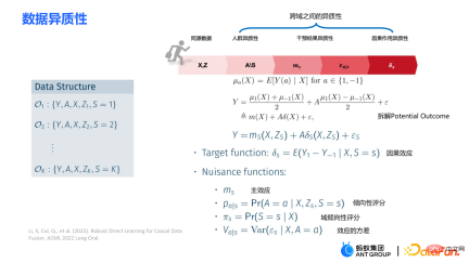



 is the causal information-aware weighting module to be mentioned later, which is a major contribution of our work; the denominator is similar to the propensity score in the doubly robust method, except that in this work both Domain information is taken into account. If the causal effects between different domains are different, the indicator information of the domain will also be considered.
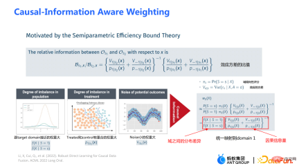
 is a module for balanced conversion of distribution differences between domains;
  is a causal information module. The three pictures on the left can be used to assist understanding: If the distribution difference between the source domain and the target domain is large, priority will be given to samples that are closer to the target domain. Weight;
4. Business applications in Ant

5. Question and Answer Session
#Q1: What are the similarities and differences between GBCT correction and double difference method (DID)?
Q2: GBCT will perform better on unobserved confounding variables. Is there any more intuitive explanation?
Q3: Have you compared GBCT with Double Machine Learning (DML)?
#Q4: A similar problem that may be encountered in business is that there may be selection bias offline. However, online bias may be somewhat different from offline bias. At this time, when doing effect evaluation offline, there may be no way to estimate the offline effect very accurately.
The above is the detailed content of How to make better use of data in causal inference?. For more information, please follow other related articles on the PHP Chinese website!
![Can't use ChatGPT! Explaining the causes and solutions that can be tested immediately [Latest 2025]](https://img.php.cn/upload/article/001/242/473/174717025174979.jpg?x-oss-process=image/resize,p_40) Can't use ChatGPT! Explaining the causes and solutions that can be tested immediately [Latest 2025]May 14, 2025 am 05:04 AM
Can't use ChatGPT! Explaining the causes and solutions that can be tested immediately [Latest 2025]May 14, 2025 am 05:04 AMChatGPT is not accessible? This article provides a variety of practical solutions! Many users may encounter problems such as inaccessibility or slow response when using ChatGPT on a daily basis. This article will guide you to solve these problems step by step based on different situations. Causes of ChatGPT's inaccessibility and preliminary troubleshooting First, we need to determine whether the problem lies in the OpenAI server side, or the user's own network or device problems. Please follow the steps below to troubleshoot: Step 1: Check the official status of OpenAI Visit the OpenAI Status page (status.openai.com) to see if the ChatGPT service is running normally. If a red or yellow alarm is displayed, it means Open
 Calculating The Risk Of ASI Starts With Human MindsMay 14, 2025 am 05:02 AM
On 10 May 2025, MIT physicist Max Tegmark told The Guardian that AI labs should emulate Oppenheimer’s Trinity-test calculus before releasing Artificial Super-Intelligence. “My assessment is that the 'Compton constant', the probability that a race to
 An easy-to-understand explanation of how to write and compose lyrics and recommended tools in ChatGPTMay 14, 2025 am 05:01 AM
AI music creation technology is changing with each passing day. This article will use AI models such as ChatGPT as an example to explain in detail how to use AI to assist music creation, and explain it with actual cases. We will introduce how to create music through SunoAI, AI jukebox on Hugging Face, and Python's Music21 library. Through these technologies, everyone can easily create original music. However, it should be noted that the copyright issue of AI-generated content cannot be ignored, and you must be cautious when using it. Let’s explore the infinite possibilities of AI in the music field together! OpenAI's latest AI agent "OpenAI Deep Research" introduces: [ChatGPT]Ope
 What is ChatGPT-4? A thorough explanation of what you can do, the pricing, and the differences from GPT-3.5!May 14, 2025 am 05:00 AM
The emergence of ChatGPT-4 has greatly expanded the possibility of AI applications. Compared with GPT-3.5, ChatGPT-4 has significantly improved. It has powerful context comprehension capabilities and can also recognize and generate images. It is a universal AI assistant. It has shown great potential in many fields such as improving business efficiency and assisting creation. However, at the same time, we must also pay attention to the precautions in its use. This article will explain the characteristics of ChatGPT-4 in detail and introduce effective usage methods for different scenarios. The article contains skills to make full use of the latest AI technologies, please refer to it. OpenAI's latest AI agent, please click the link below for details of "OpenAI Deep Research"
 Explaining how to use the ChatGPT app! Japanese support and voice conversation functionMay 14, 2025 am 04:59 AM
ChatGPT App: Unleash your creativity with the AI assistant! Beginner's Guide The ChatGPT app is an innovative AI assistant that handles a wide range of tasks, including writing, translation, and question answering. It is a tool with endless possibilities that is useful for creative activities and information gathering. In this article, we will explain in an easy-to-understand way for beginners, from how to install the ChatGPT smartphone app, to the features unique to apps such as voice input functions and plugins, as well as the points to keep in mind when using the app. We'll also be taking a closer look at plugin restrictions and device-to-device configuration synchronization
 How do I use the Chinese version of ChatGPT? Explanation of registration procedures and feesMay 14, 2025 am 04:56 AM
ChatGPT Chinese version: Unlock new experience of Chinese AI dialogue ChatGPT is popular all over the world, did you know it also offers a Chinese version? This powerful AI tool not only supports daily conversations, but also handles professional content and is compatible with Simplified and Traditional Chinese. Whether it is a user in China or a friend who is learning Chinese, you can benefit from it. This article will introduce in detail how to use ChatGPT Chinese version, including account settings, Chinese prompt word input, filter use, and selection of different packages, and analyze potential risks and response strategies. In addition, we will also compare ChatGPT Chinese version with other Chinese AI tools to help you better understand its advantages and application scenarios. OpenAI's latest AI intelligence
 5 AI Agent Myths You Need To Stop Believing NowMay 14, 2025 am 04:54 AM
These can be thought of as the next leap forward in the field of generative AI, which gave us ChatGPT and other large-language-model chatbots. Rather than simply answering questions or generating information, they can take action on our behalf, inter
 An easy-to-understand explanation of the illegality of creating and managing multiple accounts using ChatGPTMay 14, 2025 am 04:50 AM
Efficient multiple account management techniques using ChatGPT | A thorough explanation of how to use business and private life! ChatGPT is used in a variety of situations, but some people may be worried about managing multiple accounts. This article will explain in detail how to create multiple accounts for ChatGPT, what to do when using it, and how to operate it safely and efficiently. We also cover important points such as the difference in business and private use, and complying with OpenAI's terms of use, and provide a guide to help you safely utilize multiple accounts. OpenAI


Hot AI Tools

Undresser.AI Undress
AI-powered app for creating realistic nude photos

AI Clothes Remover
Online AI tool for removing clothes from photos.

Undress AI Tool
Undress images for free

Clothoff.io
AI clothes remover

Video Face Swap
Swap faces in any video effortlessly with our completely free AI face swap tool!

Hot Article

Hot Tools

MinGW - Minimalist GNU for Windows
This project is in the process of being migrated to osdn.net/projects/mingw, you can continue to follow us there. MinGW: A native Windows port of the GNU Compiler Collection (GCC), freely distributable import libraries and header files for building native Windows applications; includes extensions to the MSVC runtime to support C99 functionality. All MinGW software can run on 64-bit Windows platforms.

SublimeText3 Chinese version
Chinese version, very easy to use

DVWA
Damn Vulnerable Web App (DVWA) is a PHP/MySQL web application that is very vulnerable. Its main goals are to be an aid for security professionals to test their skills and tools in a legal environment, to help web developers better understand the process of securing web applications, and to help teachers/students teach/learn in a classroom environment Web application security. The goal of DVWA is to practice some of the most common web vulnerabilities through a simple and straightforward interface, with varying degrees of difficulty. Please note that this software

Zend Studio 13.0.1
Powerful PHP integrated development environment

PhpStorm Mac version
The latest (2018.2.1) professional PHP integrated development tool


