Seven popular reinforcement learning algorithms and code implementations

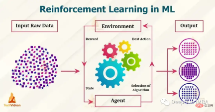
Currently popular reinforcement learning algorithms include Q-learning, SARSA, DDPG, A2C, PPO, DQN and TRPO. These algorithms have been used in various applications such as games, robots, and decision-making, and these popular algorithms are constantly being developed and improved. In this article, we will give a brief introduction to them.

1. Q-learning

Q-learning: Q-learning is a model-free, non-strategy reinforcement learning algorithm. It estimates the optimal action value function using the Bellman equation, which iteratively updates the estimated value for a given state-action pair. Q-learning is known for its simplicity and ability to handle large continuous state spaces.

The following is a simple example of using Python to implement Q-learning:

import numpy as np
 
 # Define the Q-table and the learning rate
 Q = np.zeros((state_space_size, action_space_size))
 alpha = 0.1
 
 # Define the exploration rate and discount factor
 epsilon = 0.1
 gamma = 0.99
 
 for episode in range(num_episodes):
 current_state = initial_state
 while not done:
 # Choose an action using an epsilon-greedy policy
 if np.random.uniform(0, 1) < epsilon:
 action = np.random.randint(0, action_space_size)
 else:
 action = np.argmax(Q[current_state])
 
 # Take the action and observe the next state and reward
 next_state, reward, done = take_action(current_state, action)
 
 # Update the Q-table using the Bellman equation
 Q[current_state, action] = Q[current_state, action] + alpha * (reward + gamma * np.max(Q[next_state]) - Q[current_state, action])
 
 current_state = next_state

In the above example, state_space_size and action_space_size are the number of states and actions in the environment respectively. num_episodes is the number of rounds to run the algorithm for. initial_state is the starting state of the environment. take_action(current_state, action) is a function that takes as input the current state and an action and returns the next state, reward, and a boolean indicating whether the round is complete.

In the while loop, use the epsilon-greedy strategy to select an action based on the current state. Use probability epsilon to choose a random action, and use probability 1-epsilon to choose the action with the highest Q-value for the current state.

After taking action, observe the next state and reward, and update q using the Bellman equation. and updates the current state to the next state. This is just a simple example of Q-learning and does not take into account the initialization of the Q-table and the specific details of the problem to be solved.

2. SARSA

SARSA: SARSA is a model-free, policy-based reinforcement learning algorithm. It also uses the Bellman equation to estimate the action value function, but it is based on the expected value of the next action, rather than the optimal action like in Q-learning. SARSA is known for its ability to handle stochastic dynamics problems.

import numpy as np
 
 # Define the Q-table and the learning rate
 Q = np.zeros((state_space_size, action_space_size))
 alpha = 0.1
 
 # Define the exploration rate and discount factor
 epsilon = 0.1
 gamma = 0.99
 
 for episode in range(num_episodes):
 current_state = initial_state
 action = epsilon_greedy_policy(epsilon, Q, current_state)
 while not done:
 # Take the action and observe the next state and reward
 next_state, reward, done = take_action(current_state, action)
 # Choose next action using epsilon-greedy policy
 next_action = epsilon_greedy_policy(epsilon, Q, next_state)
 # Update the Q-table using the Bellman equation
 Q[current_state, action] = Q[current_state, action] + alpha * (reward + gamma * Q[next_state, next_action] - Q[current_state, action])
 current_state = next_state
 action = next_action

state_space_size and action_space_size are the number of states and operations in the environment respectively. num_episodes is the number of rounds you want to run the SARSA algorithm. Initial_state is the initial state of the environment. take_action(current_state, action) is a function that takes the current state and the action as input and returns the next state, the reward, and a boolean indicating whether the plot is completed.

In the while loop, use the epsilon-greedy policy defined in a separate function epsilon_greedy_policy(epsilon, Q, current_state) to select actions based on the current state. Choose a random action using probability epsilon, and the action with the highest Q-value for the current state using probability 1-epsilon.

The above is the same as Q-learning, but after taking an action, it then uses a greedy strategy to choose the next action while observing the next state and reward. and update the q-table using the Bellman equation.

3. DDPG

DDPG is a model-free, non-policy algorithm for continuous action spaces. It is an actor-critic algorithm where an actor network is used to select actions and a critic network is used to evaluate actions. DDPG is particularly useful for robot control and other continuous control tasks.

import numpy as np
 from keras.models import Model, Sequential
 from keras.layers import Dense, Input
 from keras.optimizers import Adam
 
 # Define the actor and critic models
 actor = Sequential()
 actor.add(Dense(32, input_dim=state_space_size, activation='relu'))
 actor.add(Dense(32, activation='relu'))
 actor.add(Dense(action_space_size, activation='tanh'))
 actor.compile(loss='mse', optimizer=Adam(lr=0.001))
 
 critic = Sequential()
 critic.add(Dense(32, input_dim=state_space_size, activation='relu'))
 critic.add(Dense(32, activation='relu'))
 critic.add(Dense(1, activation='linear'))
 critic.compile(loss='mse', optimizer=Adam(lr=0.001))
 
 # Define the replay buffer
 replay_buffer = []
 
 # Define the exploration noise
 exploration_noise = OrnsteinUhlenbeckProcess(size=action_space_size, theta=0.15, mu=0, sigma=0.2)
 
 for episode in range(num_episodes):
 current_state = initial_state
 while not done:
 # Select an action using the actor model and add exploration noise
 action = actor.predict(current_state)[0] + exploration_noise.sample()
 action = np.clip(action, -1, 1)
 
 # Take the action and observe the next state and reward
 next_state, reward, done = take_action(current_state, action)
 
 # Add the experience to the replay buffer
 replay_buffer.append((current_state, action, reward, next_state, done))
 
 # Sample a batch of experiences from the replay buffer
 batch = sample(replay_buffer, batch_size)
 
 # Update the critic model
 states = np.array([x[0] for x in batch])
 actions = np.array([x[1] for x in batch])
 rewards = np.array([x[2] for x in batch])
 next_states = np.array([x[3] for x in batch])
 
 target_q_values = rewards + gamma * critic.predict(next_states)
 critic.train_on_batch(states, target_q_values)
 
 # Update the actor model
 action_gradients = np.array(critic.get_gradients(states, actions))
 actor.train_on_batch(states, action_gradients)
 
 current_state = next_state

In this example, state_space_size and action_space_size are the number of states and operations in the environment respectively. num_episodes is the number of rounds. Initial_state is the initial state of the environment. Take_action (current_state, action) is a function that accepts the current state and action as input and returns the next action.

4. A2C

A2C (Advantage Actor-Critic) is a strategic actor-critic algorithm that uses the Advantage function to update the strategy. The algorithm is simple to implement and can handle both discrete and continuous action spaces.

import numpy as np
 from keras.models import Model, Sequential
 from keras.layers import Dense, Input
 from keras.optimizers import Adam
 from keras.utils import to_categorical
 
 # Define the actor and critic models
 state_input = Input(shape=(state_space_size,))
 actor = Dense(32, activation='relu')(state_input)
 actor = Dense(32, activation='relu')(actor)
 actor = Dense(action_space_size, activation='softmax')(actor)
 actor_model = Model(inputs=state_input, outputs=actor)
 actor_model.compile(loss='categorical_crossentropy', optimizer=Adam(lr=0.001))
 
 state_input = Input(shape=(state_space_size,))
 critic = Dense(32, activation='relu')(state_input)
 critic = Dense(32, activation='relu')(critic)
 critic = Dense(1, activation='linear')(critic)
 critic_model = Model(inputs=state_input, outputs=critic)
 critic_model.compile(loss='mse', optimizer=Adam(lr=0.001))
 
 for episode in range(num_episodes):
 current_state = initial_state
 done = False
 while not done:
 # Select an action using the actor model and add exploration noise
 action_probs = actor_model.predict(np.array([current_state]))[0]
 action = np.random.choice(range(action_space_size), p=action_probs)
 
 # Take the action and observe the next state and reward
 next_state, reward, done = take_action(current_state, action)
 
 # Calculate the advantage
 target_value = critic_model.predict(np.array([next_state]))[0][0]
 advantage = reward + gamma * target_value - critic_model.predict(np.array([current_state]))[0][0]
 
 # Update the actor model
 action_one_hot = to_categorical(action, action_space_size)
 actor_model.train_on_batch(np.array([current_state]), advantage * action_one_hot)
 
 # Update the critic model
 critic_model.train_on_batch(np.array([current_state]), reward + gamma * target_value)
 
 current_state = next_state

In this example, the actor model is a neural network with 2 hidden layers, each with 32 neurons, with a relu activation function, and the output layer has a softmax activation function. The critic model is also a neural network with 2 hidden layers, 32 neurons in each layer, a relu activation function, and an output layer with a linear activation function.

Use the categorical cross-entropy loss function to train the actor model, and use the mean square error loss function to train the critic model. Actions are selected based on actor model predictions, with noise added for exploration.

5. PPO

PPO (Proximal Policy Optimization) is a policy algorithm that uses trust domain optimization to update the policy. It is particularly useful in environments with high-dimensional observation and continuous action spaces. PPO is known for its stability and high sample efficiency.

import numpy as np
 from keras.models import Model, Sequential
 from keras.layers import Dense, Input
 from keras.optimizers import Adam
 
 # Define the policy model
 state_input = Input(shape=(state_space_size,))
 policy = Dense(32, activation='relu')(state_input)
 policy = Dense(32, activation='relu')(policy)
 policy = Dense(action_space_size, activation='softmax')(policy)
 policy_model = Model(inputs=state_input, outputs=policy)
 
 # Define the value model
 value_model = Model(inputs=state_input, outputs=Dense(1, activation='linear')(policy))
 
 # Define the optimizer
 optimizer = Adam(lr=0.001)
 
 for episode in range(num_episodes):
 current_state = initial_state
 while not done:
 # Select an action using the policy model
 action_probs = policy_model.predict(np.array([current_state]))[0]
 action = np.random.choice(range(action_space_size), p=action_probs)
 
 # Take the action and observe the next state and reward
 next_state, reward, done = take_action(current_state, action)
 
 # Calculate the advantage
 target_value = value_model.predict(np.array([next_state]))[0][0]
 advantage = reward + gamma * target_value - value_model.predict(np.array([current_state]))[0][0]
 
 # Calculate the old and new policy probabilities
 old_policy_prob = action_probs[action]
 new_policy_prob = policy_model.predict(np.array([next_state]))[0][action]
 
 # Calculate the ratio and the surrogate loss
 ratio = new_policy_prob / old_policy_prob
 surrogate_loss = np.minimum(ratio * advantage, np.clip(ratio, 1 - epsilon, 1 + epsilon) * advantage)
 
 # Update the policy and value models
 policy_model.trainable_weights = value_model.trainable_weights
 policy_model.compile(optimizer=optimizer, loss=-surrogate_loss)
 policy_model.train_on_batch(np.array([current_state]), np.array([action_one_hot]))
 value_model.train_on_batch(np.array([current_state]), reward + gamma * target_value)
 
 current_state = next_state

6, DQN

DQN (Deep Q Network) is a model-free, non-policy algorithm that uses a neural network to approximate the Q function. DQN is particularly useful for Atari games and other similar problems where the state space is high-dimensional and neural networks are used to approximate the Q-function.

import numpy as np
 from keras.models import Sequential
 from keras.layers import Dense, Input
 from keras.optimizers import Adam
 from collections import deque
 
 # Define the Q-network model
 model = Sequential()
 model.add(Dense(32, input_dim=state_space_size, activation='relu'))
 model.add(Dense(32, activation='relu'))
 model.add(Dense(action_space_size, activation='linear'))
 model.compile(loss='mse', optimizer=Adam(lr=0.001))
 
 # Define the replay buffer
 replay_buffer = deque(maxlen=replay_buffer_size)
 
 for episode in range(num_episodes):
 current_state = initial_state
 while not done:
 # Select an action using an epsilon-greedy policy
 if np.random.rand() < epsilon:
 action = np.random.randint(0, action_space_size)
 else:
 action = np.argmax(model.predict(np.array([current_state]))[0])
 
 # Take the action and observe the next state and reward
 next_state, reward, done = take_action(current_state, action)
 
 # Add the experience to the replay buffer
 replay_buffer.append((current_state, action, reward, next_state, done))
 
 # Sample a batch of experiences from the replay buffer
 batch = random.sample(replay_buffer, batch_size)
 
 # Prepare the inputs and targets for the Q-network
 inputs = np.array([x[0] for x in batch])
 targets = model.predict(inputs)
 for i, (state, action, reward, next_state, done) in enumerate(batch):
 if done:
 targets[i, action] = reward
 else:
 targets[i, action] = reward + gamma * np.max(model.predict(np.array([next_state]))[0])
 
 # Update the Q-network
 model.train_on_batch(inputs, targets)
 
 current_state = next_state

上面的代码，Q-network有2个隐藏层，每个隐藏层有32个神经元，使用relu激活函数。该网络使用均方误差损失函数和Adam优化器进行训练。

7、TRPO

TRPO （Trust Region Policy Optimization）是一种无模型的策略算法，它使用信任域优化方法来更新策略。 它在具有高维观察和连续动作空间的环境中特别有用。

TRPO 是一个复杂的算法，需要多个步骤和组件来实现。TRPO不是用几行代码就能实现的简单算法。

所以我们这里使用实现了TRPO的现有库，例如OpenAI Baselines，它提供了包括TRPO在内的各种预先实现的强化学习算法，。

要在OpenAI Baselines中使用TRPO，我们需要安装:

pip install baselines

然后可以使用baselines库中的trpo_mpi模块在你的环境中训练TRPO代理，这里有一个简单的例子:

import gym
 from baselines.common.vec_env.dummy_vec_env import DummyVecEnv
 from baselines.trpo_mpi import trpo_mpi
 
 #Initialize the environment
 env = gym.make("CartPole-v1")
 env = DummyVecEnv([lambda: env])
 
 # Define the policy network
 policy_fn = mlp_policy
 
 #Train the TRPO model
 model = trpo_mpi.learn(env, policy_fn, max_iters=1000)

我们使用Gym库初始化环境。然后定义策略网络，并调用TRPO模块中的learn()函数来训练模型。

还有许多其他库也提供了TRPO的实现，例如TensorFlow、PyTorch和RLLib。下面时一个使用TF 2.0实现的样例

import tensorflow as tf
 import gym
 
 # Define the policy network
 class PolicyNetwork(tf.keras.Model):
 def __init__(self):
 super(PolicyNetwork, self).__init__()
 self.dense1 = tf.keras.layers.Dense(16, activation='relu')
 self.dense2 = tf.keras.layers.Dense(16, activation='relu')
 self.dense3 = tf.keras.layers.Dense(1, activation='sigmoid')
 
 def call(self, inputs):
 x = self.dense1(inputs)
 x = self.dense2(x)
 x = self.dense3(x)
 return x
 
 # Initialize the environment
 env = gym.make("CartPole-v1")
 
 # Initialize the policy network
 policy_network = PolicyNetwork()
 
 # Define the optimizer
 optimizer = tf.optimizers.Adam()
 
 # Define the loss function
 loss_fn = tf.losses.BinaryCrossentropy()
 
 # Set the maximum number of iterations
 max_iters = 1000
 
 # Start the training loop
 for i in range(max_iters):
 # Sample an action from the policy network
 action = tf.squeeze(tf.random.categorical(policy_network(observation), 1))
 
 # Take a step in the environment
 observation, reward, done, _ = env.step(action)
 
 with tf.GradientTape() as tape:
 # Compute the loss
 loss = loss_fn(reward, policy_network(observation))
 
 # Compute the gradients
 grads = tape.gradient(loss, policy_network.trainable_variables)
 
 # Perform the update step
 optimizer.apply_gradients(zip(grads, policy_network.trainable_variables))
 
 if done:
 # Reset the environment
 observation = env.reset()

在这个例子中，我们首先使用TensorFlow的Keras API定义一个策略网络。然后使用Gym库和策略网络初始化环境。然后定义用于训练策略网络的优化器和损失函数。

在训练循环中，从策略网络中采样一个动作，在环境中前进一步，然后使用TensorFlow的GradientTape计算损失和梯度。然后我们使用优化器执行更新步骤。

这是一个简单的例子，只展示了如何在TensorFlow 2.0中实现TRPO。TRPO是一个非常复杂的算法，这个例子没有涵盖所有的细节，但它是试验TRPO的一个很好的起点。

总结

以上就是我们总结的7个常用的强化学习算法，这些算法并不相互排斥，通常与其他技术(如值函数逼近、基于模型的方法和集成方法)结合使用，可以获得更好的结果。

The above is the detailed content of Seven popular reinforcement learning algorithms and code implementations. For more information, please follow other related articles on the PHP Chinese website!