 Technology peripherals
 AI
AI New perspective on image generation: discussing NeRF-based generalization methods
New perspective on image generation: discussing NeRF-based generalization methods
New perspective image generation (NVS) is an application field of computer vision. In the 1998 SuperBowl game, CMU's RI demonstrated NVS given multi-camera stereo vision (MVS). At that time, this technology was transferred to the United States A sports TV station, but it was not commercialized in the end; the British BBC Broadcasting Company invested in research and development for this, but it was not truly commercialized.
In the field of image-based rendering (IBR), there is a branch of NVS application, namely depth image-based rendering (DBIR). In addition, 3D TV, which was very popular in 2010, also needed to obtain binocular stereoscopic effects from monocular video, but due to the immaturity of the technology, it did not become popular in the end. At that time, methods based on machine learning had already begun to be researched. For example, Youtube used image search methods to synthesize depth maps.
A few years ago I introduced the application of deep learning in NVS: New perspective image generation method based on deep learning
Recent paragraph Over time, Neural Radiation Fields (NeRF) have become an effective paradigm for representing scenes and synthesizing photorealistic images, and its most direct application is NVS. A major limitation of traditional NeRF is that it is often impossible to generate high-quality renderings at new viewpoints that are significantly different from the training viewpoint. The following is a discussion of the generalization method of NeRF. The basic introduction of NeRF principles is ignored here. If you are interested, please refer to the review paper:
- Overview of Progress in Neural Rendering
-
Neural Body Rendering: NeRF and other methods
##The paper [2] proposes a universal depth The neural network MVSNeRF, achieves cross-scene generalization, inferring reconstructed radiation fields from only three nearby input views. The method utilizes plane scanned volumes (widely used in multi-view stereo vision) for geometry-aware scene reasoning and combines them with physically based volume rendering for neural radiation field reconstruction.

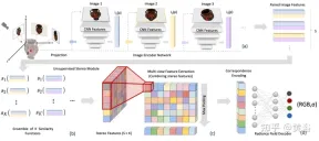
Paper [3] proposes Stereo Radiation Field (SRF), an end-to-end trained neural view synthesis method that can generalize to new scenes and only requires sparse views during testing. The core idea is a neural architecture inspired by the classic multi-view stereo (MVS) method to estimate surface points by finding similar image regions in stereo images. Input 10 views into the encoder network and extract multi-scale features. Multilayer Perceptrons (MLPs) replace classic image patch or feature matching, outputting an ensemble of similarity scores. In SRF, each 3D point is given an encoding of its stereoscopic counterpart in the input image, and its color and density are predicted in advance. This encoding is learned implicitly through the ensemble of pairwise similarities - simulating classical stereo vision.
With known camera parameters, given a set of N reference images, SRF predicts the color and density of 3D points. Construct the SRF model f, similar to the classic multi-view stereo vision method: (1) To encode the position of a point, project it into each reference view and build a local feature descriptor; (2) If On a surface and photo-consistent, feature descriptors should match each other; feature matching is simulated with a learned function that encodes the features of all reference views; (3) The encoding is decoded by a learned decoder, becoming NeRF representation. Figure 2 gives an overview of SRF: (a) extract image features; (b) simulate the process of finding photo consistency through a learned similarity function to obtain a stereoscopic feature matrix (SFM); (c) aggregate information to obtain Multi-view feature matrix (MFM); (d) Maximum pooling obtains a compact encoding of correspondence and color, which is decoded to obtain color and volume density.
The paper [4] proposes DietNeRF, a 3D neural scene representation estimated from several images. It introduces an auxiliary semantic consistency loss that encourages realistic rendering of new poses.
When only a few views are available in NeRF, the rendering problem is unconstrained; unless strictly regularized, NeRF often suffers from degenerate solutions. As shown in Figure 3: (A) When taking 100 observations of an object from uniformly sampled poses, NeRF estimates a detailed and accurate representation, allowing high-quality view synthesis purely from multi-view consistency; (B) In the case of only 8 views, placing the target in the near field of the training camera, the same NeRF overfitting leads to target misalignment and degradation in the pose near the training camera; (C) When regularization, simplification, When adjusted and re-initialized by hand, NeRF can converge but no longer captures fine details; (D) Without prior knowledge about similar objects, single-scene view synthesis cannot reasonably complete unobserved regions.

Figure 4 is a schematic diagram of the work of DietNeRF: Based on the principle of "from any angle, an object is that object", DietNeRF monitors the radiation field of any posture (DietNeRF camera ); the semantic consistency loss is calculated in the feature space that captures high-level scene attributes, not in the pixel space; so CLIP, a visual Transformer, is used to extract the semantic representation of the rendering, and then maximize the similarity with the ground truth view representation.
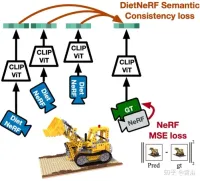
In fact, the prior knowledge of scene semantics learned by a single-view 2D image encoder can constrain a 3D representation. DietNeRF is trained from a collection of hundreds of millions of single-view 2D photos mined from the web under natural language supervision: (1) renders correctly given a given input view from the same pose, (2) matches high-level semantics across different random poses Attributes. The semantic loss function can supervise the DietNeRF model from arbitrary poses.
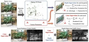
Paper [5] proposes DS-NeRF, which uses a learning radiation field loss and uses ready-made depth map supervision, as shown in Figure 5. There is the fact that current NeRF pipelines require images with known camera poses, which are typically estimated via Structure from Motion (SFM). Crucially, SFM also produces sparse 3D points that are used during training as “free” depth supervision: adding a loss that encourages a ray’s termination depth distribution to match a given 3D keypoint, including depth Uncertainty.
Paper [6] proposes pixelNeRF, a learning framework for predicting continuous neural scene representations based on one or more input images. It introduces a fully convolutional method to adjust the NeRF architecture on image input, allowing the network to be trained across multiple scenes to learn the prior knowledge of a scene, so that it can proceed from a sparse set of views (at least one) in a feed-forward manner. New view composition. Leveraging NeRF's volume rendering method, pixelNeRF can be trained directly from images without additional 3D supervision.
Specifically, pixelNeRF first calculates a fully convolutional image feature grid (feature grid) from the input image, and adjusts NeRF on the input image. Then, for each 3D query space point x and view direction d of interest in the view coordinate system, the corresponding image features are sampled via projection and bilinear interpolation. The query specification is sent along with the image features to the NeRF network which outputs density and color, where the spatial image features are fed as a residual to each layer. When multiple images are available, the input is first encoded into a latent representation of each camera coordinate system, which is merged in an intermediate layer before predicting color and density. The model training is based on the reconstruction loss between a ground truth image and a volume rendered view. The
pixelNeRF framework is shown in Figure 6: For a 3D query point x along the view direction d, of a target camera ray, from the feature volume W## through projection and interpolation #Extract the corresponding image features; then pass the features together with the spatial coordinates to the NeRF networkf; the output RGB and density values are used for volume rendering and compared with the target pixel value; the coordinates x and dIn the camera coordinate system of the input view.

Image-based rendering (IBR) work. Unlike neural scene representations, which optimize each scene function for rendering, IBRNet learns a general view interpolation function that generalizes to new scenes. Still using classic volume rendering to synthesize images, it is fully differentiable and trained with multi-view pose images as supervision.
The light transformer considers these density features along the entire ray to calculate the scalar density value of each sample, enabling visibility reasoning on larger spatial scales. Separately, a color blending module derives the view-dependent color of each sample using the 2D features and the source view's sight vector. Finally, volume rendering calculates the final color value for each ray. Figure 7 is an overview of IBRNet: 1) To render the target view (marked "?" image), first identify a set of adjacent source views (for example, views marked A and B) and extract the images Features; 2) Then, for each ray in the target view, use IBRNet (yellow shaded area) to calculate a set of sample colors and densities along the ray; specifically, for each sample, aggregate the corresponding color and density from the adjacent source view information (image color, features, and viewing direction) to generate its color and density features; then, a ray transformer is applied to the density features of all samples on the ray to predict density values. 3) Finally, use volume rendering to accumulate color and density along the ray. On the reconstructed image color, end-to-end L2 loss training can be performed.
Figure 8 shows the color volume density prediction work of IBRNet for continuous 5D positions: first, the 2D image features extracted from all source views are input into an MLP similar to PointNet, and local and global information are aggregated to generate multi-view perceptual features. And pooling weights, use weights to concentrate features, perform multi-view visibility reasoning, and obtain density features; instead of directly predicting the density σ of a single 5D sample, the ray transformer module is used to gather all sample information along the ray; ray transformer The module obtains density features for all samples on the ray and predicts its density; the ray transformer module enables geometric reasoning over longer ranges and improves density prediction; for color prediction, multi-view perception features are combined with the query ray relative to the source The viewing direction of the view is connected to the input of a small network to predict a set of harmonic weights. The output color c is the weighted average of the image color of the source view.
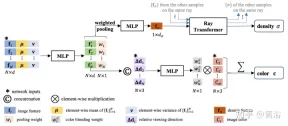
One more thing to add here: Unlike NeRF which uses the absolute viewing direction, IBRNet considers the viewing direction relative to the source view, that is, d and The difference between di, Δd=d−di. Δd is smaller, which usually means that the color of the target view is more likely to be similar to the corresponding color of the source view i, and vice versa.
The General Radiation Field (GRF) proposed in paper [8] only characterizes and renders 3D targets and scenes from 2D observations. The network models 3D geometry as a universal radiation field, takes a set of 2D images, camera extrinsic poses, and intrinsic parameters as input, builds an internal representation for each point in 3D space, and then renders the corresponding appearance and geometry viewed from any position. The key is to learn the local features of each pixel of a 2D image and then project these features to 3D points, thereby generating a versatile and rich point representation. Furthermore, an attention mechanism is integrated to aggregate pixel features of multiple 2D views to implicitly consider visual occlusion issues.
Figure 9 is a schematic diagram of GRF: GRF projects each 3D point p to each of the M input images, collecting each The features of the pixels are aggregated and fed to the MLP, which infers the color and volume density of p.

GRF consists of four parts: 1) feature extractor for each 2D pixel, a CNN-based encoder-decoder; 2) 2D feature conversion into 3D space reprojection; 3) Attention-based aggregator to obtain universal features of 3D points; 4) Neural renderer NeRF.
Since there is no depth value paired with the RGB image, there is no way to determine which specific 3D surface point the pixel feature belongs to. In the reprojection module, pixel features are considered as representations of each position along the ray in 3D space. Formally, given a 3D point, an observing 2D view, and camera pose and intrinsic parameters, the corresponding 2D pixel features can be retrieved through a reprojection operation.
In the feature aggregator, the attention mechanism learns unique weights for all input features and then aggregates them together. Through an MLP, the color and volume density of 3D points can be inferred.
Paper [9] proposes RegNeRF to regularize the geometry and appearance of image patches rendered from unobserved viewpoints, and anneal the light sampling space during training. Additionally, a normalized flow model is used to regularize the colors of unobserved viewpoints.
Figure 10 is an overview of the RegNeRF model: given a set of input images (blue camera), NeRF optimizes the reconstruction loss; however, for sparse inputs, this leads to degenerate solutions; this work is useful for future Observed views (red camera) are sampled and image patches rendered from these views are regularized for geometry and appearance; more specifically, for a given radiation field, a ray is cast through the scene and image patches are rendered from an unobserved viewpoint ; Then, the predicted RGB image patches are fed through the trained normalized flow model and the predicted log-likelihood is maximized, thereby regularizing the appearance; a smoothness loss is forced on the rendered depth patches, which can be regularized Geometry; the method leads to 3D consistent representations even for sparse inputs that render realistic new views.

The paper [10] studies a method of new view extrapolation instead of few-sample image synthesis, that is, (1) the training image can describe the target well, ( 2) There is a significant difference between the distribution of training viewpoints and testing viewpoints, which is called RapNeRF (RAy Priors NeRF).
The insight of paper [10] is that the inherent appearance of any visible projection of a 3D surface should be consistent. Therefore, it proposes a random ray casting strategy that allows unseen views to be trained with seen views. Additionally, the rendering quality of the extrapolated view can be further improved based on a precomputed ray atlas along the line of sight of the observation ray. A major limitation is that RapNeRF exploits multi-view consistency to eliminate the effect of strong view correlation.
The intuitive explanation of the random ray casting strategy is shown in Figure 11: In the left picture, there are two rays observing the 3-D point v, r1 is located in the training space, and r2 is far away from the training ray; consider Distribution drift and mapping function to NeRF Fc:(r,f)→c whose some sample radiance along r2 will be inaccurate; radiance accumulation operation along r2 compared to pixel color More likely to provide an inverse color estimate of v; the middle image is a simple virtual view reprojection that follows the NeRF formula to calculate the pixel rays involved, finding the ray corresponding to the virtual ray hitting the same 3D point from the training ray pool , very inconvenient in practice; in the picture on the right, for a specific training ray (projected from o and passing through v), Random Ray Casting (RRC) strategy randomly generates an unseen ray within a cone A virtual ray (projected from o′ and through v) is then assigned a pseudo label online based on the training ray; RRC supports training unseen rays with seen rays.

#RRC strategy allows assigning pseudo-labels to randomly generated virtual rays in an online manner. Specifically, for a pixel of interest in a training image I, the observation direction d, camera origin o and depth in its world coordinate system are given The value is tz , and the ray r=o td . Here, tz is precomputed and stored using pretrained NeRF.
Suppose v=o tzd represents the nearest 3D surface point hit by r. During the training phase, v is regarded as the new origin, and a ray is randomly cast from v within the cone, whose center line is the vector vo¯=− tzd. This can be easily achieved by converting vo¯ to spherical space and introducing some random perturbations Δφ and Δθ to φ and θ. Here, φ and θ are the azimuth angle and elevation angle of vo¯ respectively. Δφ and Δθ are sampled uniformly from the predefined interval [−η, η]. From this we get θ′=θ Δθ and φ′=φ Δφ. Therefore, a virtual ray can be cast from a random origin o' that also passes through v. In this way, the true value of the color intensity I(r) can be regarded as a pseudo token of I~(r′).
Basic NeRF utilizes "directional embedding" to encode the lighting effects of the scene. The scene fitting process makes the trained color prediction MLP heavily dependent on the gaze direction. For new view interpolation this is not a problem. However, this may not be suitable for new view extrapolation due to some differences between training and test light distributions. A naive idea would be to simply remove the directional embedding (denoted as "NeRF w/o dir"). However, this often produces image artifacts such as unexpected ripples and non-smooth colors. This means that the viewing direction of light may also be related to surface smoothness.
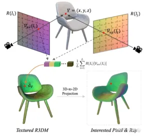
The paper [10] calculates a ray atlas and shows that it can further improve the rendering quality of extrapolated views without involving the problem of interpolated views. A ray atlas is similar to a texture atlas, but it stores the global ray direction for each 3D vertex.
In particular, for each image (e.g., image I), the viewing directions of its rays are grabbed for all spatial locations, thereby generating a ray map. Extract a rough 3D mesh (R3DM) from pre-trained NeRF and map ray directions to 3D vertices. Taking vertex V=(x,y,z) as an example, its global light direction d¯V should be expressed as
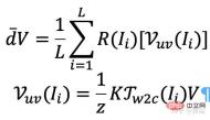
Where K is the internal parameter of the camera, Γw2c(Ii) is the camera-world coordinate system transformation matrix of the image Ii, Vuv(Ii) is the 2-D projected position of vertex V in image Ii, and L is the number of training images in vertex V reconstruction. For each pixel of an arbitrary camera pose, projecting a 3D mesh with a light map texture (R3DM) to 2D can obtain a global ray prior d¯ .
Figure 12 is a schematic diagram of the light atlas: that is, capturing a light atlas from the training light and using it to add texture to the rough 3D mesh (R3DM) of the chair; R( Ii) is the light map of the training image Ii.
When training RapNeRF, use d¯ of the pixel of interest I(r) to replace its Fc d in , perform color prediction. The probability of this alternative mechanism occurring is 0.5. During the testing phase, the radiance c of sample x is approximately:

where the mapping function Fσ( x):x→(σ,f).
Original NeRF optimizes each scene representation independently, without the need to explore shared information between scenes, and is time-consuming. To solve this problem, researchers have proposed models such as PixelNeRF and MVSNeRF, which receive multiple observer views as conditional input and learn a universal neural radiation field. Following the divide-and-conquer design principle, it consists of two independent components: a CNN feature extractor for a single image and an MLP as a NeRF network. For single-view stereo vision, in these models, a CNN maps the image to a feature grid and the MLP maps the query 5D coordinates and their corresponding CNN features to a single volume density and view-dependent RGB color. For multi-view stereo vision, since CNN and MLP cannot handle any number of input views, the coordinates and corresponding features in each view's coordinate system are first processed independently, and image-conditioned intermediate representations of each view are obtained. Next, an auxiliary pooling-based model is used to aggregate the view intermediate representations within these NeRF networks. In 3D understanding tasks, multiple views provide additional information about the scene.
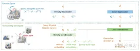
The paper [11] proposes an encoder-decoder Transformer framework TransNeRF to characterize the neural radiation field scene. TransNeRF can explore deep relationships between multiple views and aggregate multi-view information into coordinate-based scene representations through a single Transformer-based NeRF attention mechanism. In addition, TransNeRF considers the corresponding information of raycast space and peripheral view space to learn the local geometric consistency of shape and appearance in the scene.
As shown in Figure 13, TransNeRF renders the queried 3D point in a target viewing ray. TransNeRF includes: 1) In the peripheral space, the density-view decoder (Density-ViewDecoder) and the Color-ViewDecoder (Color-ViewDecoder) fuses the source view and query space information((x,y,z),d) into the latent density and color representation of the 3D query point; 2) In the ray casting space, the density ray decoder (Density-RayDecoder) and the color ray decoder (Color-RayDecoder) are used to enhance the query density and color representation by considering adjacent points along the target view ray. Finally, the volume density and directional color of the query 3D point on the target line of sight are obtained from TransNeRF.
The paper [12] proposes a generalizable NVS method with sparse input, called FWD, which provides high-quality image synthesis in real time. With explicit depth and differential rendering, FWD achieves 130-1000 times faster speeds and better perceived quality. If there is seamless integration of sensor depth during training or inference, image quality can be improved while maintaining real-time speed.
The key insight is that explicitly characterizing the depth of each input pixel allows forward warping to be applied to each input view with a differentiable point cloud renderer. This avoids the expensive volume sampling of NeRF-like methods and achieves real-time speed while maintaining high image quality.
SynSin[1] uses a differentiable point cloud renderer for single-image new view synthesis (NVS). Paper [12] extends SynSin to multiple inputs and explores effective methods to fuse multi-view information.
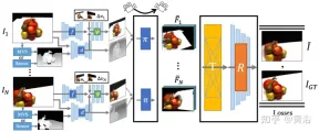
FWD estimates the depth of each input view, constructs a point cloud of latent features, and then synthesizes the new view through a point cloud renderer. In order to alleviate the inconsistency problem between observations from different viewpoints, viewpoint-related feature MLP is introduced into the point cloud to model viewpoint-related results. Another Transformer-based fusion module effectively combines features from multiple inputs. A refinement module that can inpaint missing areas and further improve composition quality. The entire model is trained end-to-end, minimizing photometric and perceptual losses, learning depth and features that optimize synthesis quality.
Figure 14 is an overview of FWD: given a set of sparse images, use feature network f (based on BigGAN architecture), view-related feature MLP ψ and depth The network d builds a point cloud (including the geometric and semantic information of the view) for each image Ii Pi; except for the image, d Take MVS (based on PatchmatchNet) estimated depth or sensor depth as input and regress the refined depth; based on image features Fi and relative view changes Δv (based on normalization View direction vi and vt, that is, from the point to the center of the input view i and target view t), through fandψregression pixel-by-pixel featuresFi′; using a differentiable point cloud renderer π (splatting) to project the point cloud and Render to the target view, i.e. F~i ; instead of directly aggregating the view point cloud before rendering, the Transformer T fuses the rendering results from any number of inputs and applies the refinement module RDecoding generates the final image result, that is, semantically and geometrically repairs unseen areas of the input, corrects local errors caused by inaccurate depth, and improves perceptual quality based on the semantics contained in the feature map; model Training uses photometric loss and content loss.
Existing methods use local image features to reconstruct 3D objects, projecting input image features on query 3D points to predict color and density, thereby inferring 3D shape and appearance. These image conditional models work well for rendering target perspective maps that are close to the input perspective. However, when the target perspective moves too much, this method leads to significant occlusion of the input view, a sharp drop in rendering quality, and blurred predictions.
In order to solve the above problem, paper [13] proposes a method that uses global and local features to form a compressed 3D representation. Global features are learned from a visual Transformer, while local features are extracted from a 2D convolutional network. To synthesize a new view, an MLP network is trained to achieve volume rendering based on the learned 3D representation. This representation enables the reconstruction of unseen regions without the need for enforced constraints such as symmetry or canonical coordinate systems.
Given a single image Is at camera s, the task is to synthesize a new view It at camera t. If a 3D point x is visible in the source image, its color Is(π(x)) can be used directly, where π represents projection in the source view, indicating that the point is visible in a new view. If x is occluded, resort to information other than the projected π(x) color. As shown in Figure 15, there are three possible solutions to obtain this kind of information: (a) General NeRF is a 1D latent code-based method that encodes 3D target information in 1D vectors. Since different 3D points share the same code, the inductive bias is Limitations; (b) 2D image-based methods reconstruct any 3D point from pixel-by-pixel image features. Such representations encourage better rendering quality in visible areas and are more computationally efficient, but rendering becomes blurry for unseen areas; (c) ) The 3D voxel-based method treats the 3-D target as a collection of voxels, and applies 3-D convolution to generate the color RGB and density vector σ, which renders faster and makes full use of 3D priors to render the unseen geometry, but rendering resolution is limited due to voxel size and limited receptive fields.
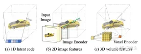
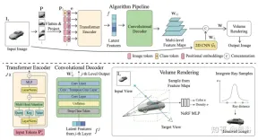
Figure 6 is an overview of the global-local hybrid rendering method [13]: First, the input image is divided into N=8×8 image blocksP; Each image patch is flattened and linearly projected to the image token (token) P1; the transformer encoder takes the image token and the learnable position embedding e as input, and extracts global information as a set of latent features f; Then, use a convolutional decoder to decode the latent features into a multi-level feature map WG; In addition to global features, use another 2D CNN model to obtain local image features; Finally, use The NeRF MLP model samples features for volume rendering.
The paper [14] proposes Point-NeRF, which combines the advantages of NeRF and MVS and uses neural 3D point clouds and related neural features to model the radiation field. Point-NeRF can be effectively rendered by aggregating neural point features near the scene surface in a ray marching-based rendering pipeline. In addition, direct inference from a pre-trained deep network initializes Point-NeRF to generate a neural point cloud; the point cloud can be fine-tuned to exceed the visual quality of NeRF and train 30 times faster. Point-NeRF is combined with other 3D reconstruction methods and adopts a growing and pruning mechanism, that is, growing in high volume density areas and pruning in low volume density, to optimize the reconstructed point cloud data.
An overview of Point-NeRF is shown in Figure 17: (a) From multi-view images, Point-NeRF generates depth for each view with a cost volume-based 3D CNN and 2D CNN from the input image. Extract 2D features; after aggregating the depth map, a point-based radiation field is obtained, where each point has a spatial position, confidence, and unprojected image features; (b) To synthesize a new view, differentiable ray travel is performed and only Calculate light and dark near the neural point cloud; at each light and dark position, Point-NeRF aggregates features from its K neural point neighbors and calculates radiance and volume density, then sums the radiance with volume density accumulation. The entire process is end-to-end trainable, and point-based radiation fields can be optimized through rendering losses.

GRAF (Generative Radiance Field)[18] is a generation model of radiation field, which is achieved by introducing a discriminator based on multi-scale patches. Synthesis of high-resolution 3D-aware images while model training requires only 2D images taken by cameras of unknown poses.
The goal is to learn a model to synthesize new scenes by training on unprocessed images. More specifically, an adversarial framework is utilized to train a generative model of radiation fields (GRAF).
Figure 18 shows an overview of the GRAF model: the generator adopts camera matrix K, camera pose ξ, 2D sampling mode ν and shape/appearance code as input and predict an image patch P′; the discriminator will synthesize the patch P ′ is compared with the patch P extracted from the real image I; during inference, for each Predict a color value for each image pixel; however, this operation is too expensive at training time, so a fixed patch of size K×K pixels is predicted, with random scaling and rotation, for the entire Radiation fields provide gradients.

Determine the center and scale s to generate the virtual K×K patch. The random patch centers come from a uniform distribution over the image domain Ω, while the patch scales s come from a uniform distribution, where W and H represent the width and height of the target image. The shape and appearance variables are sampled from the shape and appearance distributions and , respectively. In the experiments, both and use the standard Gaussian distribution.
The radiation field is represented by a deep fully connected neural network, where the parameter θ maps the position encoding of the 3D position x and the viewing direction d To RGB color valuec and volume density σ:

here gθ depends Two additional latent codes: a shape code zs determines the target shape, and an appearance code za determines the appearance. Here gθ is called the conditional radiation field, and its structure is shown in Figure 19: First, the shape code # is calculated based on the position code and shape code of x ##h; Density headσθconverts this encoding to volume densityσ; to predict the color at the 3D position xc, encode the position of h and d and the apparent code za are concatenated and the resulting vector is passed to the color header cθ; σ is calculated independently of the viewpoint d and appearance code, encouraging multi-view consistency, At the same time, shape and appearance are separated; this encourages the network to use two latent codes to model shape and appearance separately, and allows them to be processed separately during inference.

The discriminator is implemented as a convolutional neural network, which combines the predicted patch P′ with the slave data distribution pD The patch P extracted from the real image I is compared. To extract a K×K patch from a real image I, first extract pv from the same distribution used to extract the above generator patch Extract v=(u,s); then, query I at the 2D image coordinate P(u,s) through bilinear interpolation, and sample the real patch P. Use Γ(I,v) to represent this bilinear sampling operation.
Experiments found that a single discriminator with shared weights is sufficient for all patches, even if these patches are sampled at random locations at different scales. Note: The scale determines the receptive field of the patch. Therefore, to facilitate training, start with a larger receptive field patch to capture the global context. Then, patches with smaller receptive fields are progressively sampled to refine local details.
GIRAFFE[19] is used to generate scenes in a controllable and realistic way when training on raw unstructured images. The main contributions are in two aspects: 1) The combined 3D scene representation is directly incorporated into the generative model to achieve more controllable image synthesis. 2) Combine this explicit 3D representation with a neural rendering pipeline to enable faster inference and more realistic images. To this end, the scene representation is combined to generate a neural feature field, as shown in Figure 20: For a randomly sampled camera, a feature image of the scene is volume-rendered based on a separate feature field; the 2D neural rendering network will The feature image is converted into an RGB image; only the original image is used during training, and the image formation process can be controlled during testing, including camera pose, target pose, and the shape and appearance of the target; in addition, the model is expanded beyond the scope of the training data, for example, Scenes containing more objects than in the training images can be synthesized.
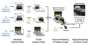
Rendering the scene volume into a relatively low-resolution feature image saves time and computation. The neural renderer processes these feature images and outputs the final render. In this way, the method can obtain high-quality images and scale to real scenes. When trained on a collection of raw unstructured images, this method allows controllable image synthesis of single- and multi-object scenes.
When combining scenes, two situations should be considered: N fixed and N changing (the last one is the background). In practice, the background is represented using the same representation as the target, except that the scale and translation parameters are fixed across the entire scene and centered around the scene space origin.
The weight of the 2D rendering operator maps the feature image to the final synthetic image, which can be parameterized as a 2D CNN with leaky ReLU activation, and combined with 3x 3 convolution and nearest neighbor upsampling to increase spatial resolution Rate. The last layer applies the sigmoid operation to get the final image prediction. Its schematic diagram is shown in Figure 21.
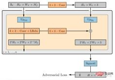
The discriminator is also a CNN with leaky ReLU activation.
The above is the detailed content of New perspective on image generation: discussing NeRF-based generalization methods. For more information, please follow other related articles on the PHP Chinese website!
 The AI Skills Gap Is Slowing Down Supply ChainsApr 26, 2025 am 11:13 AM
The term "AI-ready workforce" is frequently used, but what does it truly mean in the supply chain industry? According to Abe Eshkenazi, CEO of the Association for Supply Chain Management (ASCM), it signifies professionals capable of critic
 How One Company Is Quietly Working To Transform AI ForeverApr 26, 2025 am 11:12 AM
The decentralized AI revolution is quietly gaining momentum. This Friday in Austin, Texas, the Bittensor Endgame Summit marks a pivotal moment, transitioning decentralized AI (DeAI) from theory to practical application. Unlike the glitzy commercial
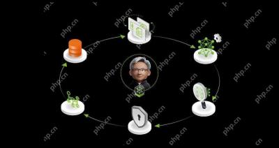 Nvidia Releases NeMo Microservices To Streamline AI Agent DevelopmentApr 26, 2025 am 11:11 AM
Enterprise AI faces data integration challenges The application of enterprise AI faces a major challenge: building systems that can maintain accuracy and practicality by continuously learning business data. NeMo microservices solve this problem by creating what Nvidia describes as "data flywheel", allowing AI systems to remain relevant through continuous exposure to enterprise information and user interaction. This newly launched toolkit contains five key microservices: NeMo Customizer handles fine-tuning of large language models with higher training throughput. NeMo Evaluator provides simplified evaluation of AI models for custom benchmarks. NeMo Guardrails implements security controls to maintain compliance and appropriateness
 AI Paints A New Picture For The Future Of Art And DesignApr 26, 2025 am 11:10 AM
AI: The Future of Art and Design Artificial intelligence (AI) is changing the field of art and design in unprecedented ways, and its impact is no longer limited to amateurs, but more profoundly affecting professionals. Artwork and design schemes generated by AI are rapidly replacing traditional material images and designers in many transactional design activities such as advertising, social media image generation and web design. However, professional artists and designers also find the practical value of AI. They use AI as an auxiliary tool to explore new aesthetic possibilities, blend different styles, and create novel visual effects. AI helps artists and designers automate repetitive tasks, propose different design elements and provide creative input. AI supports style transfer, which is to apply a style of image
 How Zoom Is Revolutionizing Work With Agentic AI: From Meetings To MilestonesApr 26, 2025 am 11:09 AM
Zoom, initially known for its video conferencing platform, is leading a workplace revolution with its innovative use of agentic AI. A recent conversation with Zoom's CTO, XD Huang, revealed the company's ambitious vision. Defining Agentic AI Huang d
 The Existential Threat To UniversitiesApr 26, 2025 am 11:08 AM
Will AI revolutionize education? This question is prompting serious reflection among educators and stakeholders. The integration of AI into education presents both opportunities and challenges. As Matthew Lynch of The Tech Edvocate notes, universit
 The Prototype: American Scientists Are Looking For Jobs AbroadApr 26, 2025 am 11:07 AM
The development of scientific research and technology in the United States may face challenges, perhaps due to budget cuts. According to Nature, the number of American scientists applying for overseas jobs increased by 32% from January to March 2025 compared with the same period in 2024. A previous poll showed that 75% of the researchers surveyed were considering searching for jobs in Europe and Canada. Hundreds of NIH and NSF grants have been terminated in the past few months, with NIH’s new grants down by about $2.3 billion this year, a drop of nearly one-third. The leaked budget proposal shows that the Trump administration is considering sharply cutting budgets for scientific institutions, with a possible reduction of up to 50%. The turmoil in the field of basic research has also affected one of the major advantages of the United States: attracting overseas talents. 35
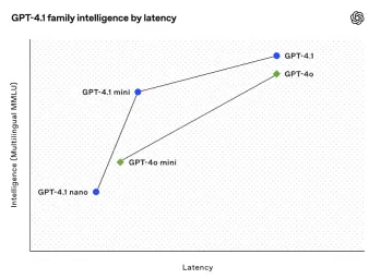 All About Open AI's Latest GPT 4.1 Family - Analytics VidhyaApr 26, 2025 am 10:19 AM
OpenAI unveils the powerful GPT-4.1 series: a family of three advanced language models designed for real-world applications. This significant leap forward offers faster response times, enhanced comprehension, and drastically reduced costs compared t


Hot AI Tools

Undresser.AI Undress
AI-powered app for creating realistic nude photos

AI Clothes Remover
Online AI tool for removing clothes from photos.

Undress AI Tool
Undress images for free

Clothoff.io
AI clothes remover

Video Face Swap
Swap faces in any video effortlessly with our completely free AI face swap tool!

Hot Article

Hot Tools

Dreamweaver CS6
Visual web development tools

SublimeText3 English version
Recommended: Win version, supports code prompts!

mPDF
mPDF is a PHP library that can generate PDF files from UTF-8 encoded HTML. The original author, Ian Back, wrote mPDF to output PDF files "on the fly" from his website and handle different languages. It is slower than original scripts like HTML2FPDF and produces larger files when using Unicode fonts, but supports CSS styles etc. and has a lot of enhancements. Supports almost all languages, including RTL (Arabic and Hebrew) and CJK (Chinese, Japanese and Korean). Supports nested block-level elements (such as P, DIV),

EditPlus Chinese cracked version
Small size, syntax highlighting, does not support code prompt function

SAP NetWeaver Server Adapter for Eclipse
Integrate Eclipse with SAP NetWeaver application server.


