

Deep reinforcement learning tackles real-world autonomous driving

arXiv paper "Tackling Real-World Autonomous Driving using Deep Reinforcement Learning", uploaded on July 5, 2022, the author is from Vislab of the University of Parma in Italy and Ambarella (acquisition of Vislab).
In a typical autonomous driving assembly line, the control system represents the two most critical components, in which data retrieved by sensors and data processed by perception algorithms are used to achieve safety Comfortable self-driving behavior. In particular, the planning module predicts the path the self-driving car should follow to perform the correct high-level actions, while the control system performs a series of low-level actions, controlling steering, throttle, and braking.
This work proposes a model-free Deep Reinforcement Learning (DRL) planner to train a neural network to predict acceleration and steering angle, thereby obtaining an autonomous The data driven by the car's positioning and perception algorithms outputs the data driven by the individual modules of the vehicle. In particular, the system that has been fully simulated and trained can drive smoothly and safely in simulated and real (Palma city area) barrier-free environments, proving that the system has good generalization capabilities and can also drive in environments other than training scenarios. In addition, in order to deploy the system on real autonomous vehicles and reduce the gap between simulated performance and real performance, the authors also developed a module represented by a miniature neural network that is able to reproduce the behavior of the real environment during simulation training. Car dynamic behavior.
Over the past few decades, tremendous progress has been made in improving the level of vehicle automation, from simple, rule-based approaches to implementing AI-based intelligent systems. In particular, these systems aim to address the main limitations of rule-based approaches, namely the lack of negotiation and interaction with other road users and the poor understanding of scene dynamics.
Reinforcement Learning (RL) is widely used to solve tasks that use discrete control space outputs, such as Go, Atari games, or chess, as well as autonomous driving in continuous control space. In particular, RL algorithms are widely used in the field of autonomous driving to develop decision-making and maneuver execution systems, such as active lane changes, lane keeping, overtaking maneuvers, intersections and roundabout processing, etc.
This article uses a delayed version of D-A3C, which belongs to the so-called Actor-Critics algorithm family. Specifically composed of two different entities: Actors and Critics. The purpose of the Actor is to select the actions that the agent must perform, while the Critics estimate the state value function, that is, how good the agent's specific state is. In other words, Actors are probability distributions π(a|s; θπ) over actions (where θ are network parameters), and critics are estimated state value functions v(st; θv) = E(Rt|st), where R is Expected returns.
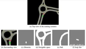
The internally developed high-definition map implements the simulation simulator; an example of the scene is shown in Figure a, which is a partial map area of the real self-driving car test system, while Figure B shows the surrounding view perceived by the agent, Corresponding to an area of 50 × 50 meters, it is divided into four channels: obstacles (Figure c), drivable space (Figure d), the path that the agent should follow (Figure e) and the stop line (Figure f). The high-definition map in the simulator allows retrieving multiple pieces of information about the external environment, such as location or number of lanes, road speed limits, etc.
Focus on achieving a smooth and safe driving style, so the agent is trained in static scenarios, excluding obstacles or other road users, learning to follow routes and respect speed limits .
Use the neural network as shown in the figure to train the agent and predict the steering angle and acceleration every 100 milliseconds. It is divided into two sub-modules: the first sub-module can define the steering angle sa, and the second sub-module is used to define the acceleration acc. The inputs to these two submodules are represented by 4 channels (drivable space, path, obstacle and stop line), corresponding to the agent's surrounding view. Each visual input channel contains four 84×84 pixel images to provide the agent with a history of past states. Along with this visual input, the network receives 5 scalar parameters, including the target speed (road speed limit), the agent's current speed, the current speed-target speed ratio, and the final action related to steering angle and acceleration.
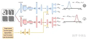
In order to ensure exploration, two Gaussian distributions are used to sample the output of the two sub-modules to obtain the relative acceleration (acc=N (μacc, σacc)) and steering Angle (sa=N(μsa,σsa)). The standard deviations σacc and σsa are predicted and modulated by the neural network during the training phase to estimate the uncertainty of the model. In addition, the network uses two different reward functions R-acc-t and R-sa-t, related to acceleration and steering angle respectively, to generate corresponding state value estimates (vacc and vsa).
The neural network was trained on four scenes in the city of Palma. For each scenario, multiple instances are created, and the agents are independent of each other on these instances. Each agent follows the kinematic bicycle model, with a steering angle of [-0.2, 0.2] and an acceleration of [-2.0 m, 2.0 m]. At the beginning of the segment, each agent starts driving at a random speed ([0.0, 8.0]) and follows its intended path, adhering to road speed limits. Road speed limits in this urban area range from 4 ms to 8.3 ms.
Finally, since there are no obstacles in the training scene, the clip can end in one of the following terminal states:
- Achieving the goal: The intelligence reaches the end target location.
- DRIVING OFF THE ROAD: The agent goes beyond its intended path and incorrectly predicts the steering angle.
- Time's Up: The time to complete the fragment has expired; this is primarily due to cautious predictions of acceleration output while driving below the road speed limit.
In order to obtain a strategy that can successfully drive a car in simulated and real environments, reward shaping is crucial to achieve the desired behavior. In particular, two different reward functions are defined to evaluate the two actions respectively: R-acc-t and R-sa-t are related to acceleration and steering angle respectively, defined as follows:
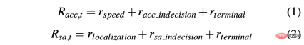
where


R-sa-t and R-acc-t both have an element in the formula for Penalize two consecutive actions whose differences in acceleration and steering angle are greater than a certain threshold δacc and δsa respectively. In particular, the difference between two consecutive accelerations is calculated as follows: Δacc=| acc (t) − acc (t− 1) | , while rac_indecision is defined as:

In contrast, the difference between two consecutive predictions of steering angle is calculated as Δsa=| sa(t)−sa(t− 1)|, while rsa_indecision is defined as follows:

Finally, R-acc-t and R-sa-t depend on the terminal state achieved by the agent:
- Goal achieved: The agent reaches the goal position, so the two rewards rterminal is set to 1.0;
- DRIVE OFF ROAD: The agent deviates from its path, mainly due to inaccurate prediction of steering angle. Therefore, assign a negative signal -1.0 to Rsa,t and a negative signal 0.0 to R-acc-t;
- Time is up: the available time to complete the segment expires, mainly due to the agent's acceleration prediction being too Be cautious; therefore, rterminal assumes −1.0 for R-acc-t and 0.0 for R-sa-t.
One of the main problems associated with simulators is the difference between simulated and real data, which is caused by the difficulty of truly reproducing real-world conditions within the simulator. To overcome this problem, a synthetic simulator is used to simplify the input to the neural network and reduce the gap between simulated and real data. In fact, the information contained in the 4 channels (obstacles, driving space, path and stop line) as input to the neural network can be easily reproduced by perception and localization algorithms and high-definition maps embedded on real autonomous vehicles.
In addition, another related issue with using simulators has to do with the difference in the two ways in which the simulated agent performs the target action and the self-driving car performs the command. In fact, the target action calculated at time t can ideally take effect immediately at the same precise moment in the simulation. The difference is that this does not happen on a real vehicle, because the reality is that such target actions will be executed with some dynamics, resulting in an execution delay (t δ). Therefore, it is necessary to introduce such response times in simulations in order to train agents on real self-driving cars to handle such delays.
To this end, in order to achieve more realistic behavior, the agent is first trained to add a low-pass filter to the neural network predicted target actions that the agent must perform. As shown in the figure, the blue curve represents the ideal and instantaneous response times occurring in the simulation using the target action (the steering angle of its example). Then, after introducing a low-pass filter, the green curve identifies the simulated agent response time. In contrast, the orange curve shows the behavior of an autonomous vehicle performing the same steering maneuver. However, it can be noticed from the figure that the difference in response time between simulated and real vehicles is still relevant.
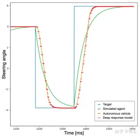
In fact, the acceleration and steering angle points preset by the neural network are not feasible commands, and do not consider some factors, such as the inertia of the system, the delay of the actuator and other non-ideal factors. Therefore, in order to reproduce the dynamics of a real vehicle as realistically as possible, a model consisting of a small neural network consisting of 3 fully connected layers (deep response) was developed. The graph of the depth response behavior is shown as the red dashed line in the figure above, and it can be noticed that it is very similar to the orange curve representing a real self-driving car. Given that the training scene is devoid of obstacles and traffic vehicles, the described problem is more pronounced for steering angle activity, but the same idea has been applied to acceleration output.
Train a deep response model using a dataset collected on a self-driving car, where the inputs correspond to the commands given to the vehicle by the human driver (accelerator pressure and steering wheel turns) and the outputs correspond to the vehicle's throttle, braking and bending , can be measured using GPS, odometer or other technology. In this way, embedding such models in a simulator results in a more scalable system that reproduces the behavior of autonomous vehicles. The depth response module is therefore essential for the correction of steering angle, but even in a less obvious way, it is necessary for acceleration, and this will become clearly visible with the introduction of obstacles.
Two different strategies were tested on real data to verify the impact of the deep response model on the system. Subsequently, verify that the vehicle follows the path correctly and adheres to the speed limits derived from the HD map. Finally, it is proven that pre-training the neural network through Imitation Learning can significantly shorten the total training time.
The strategy is as follows:
- Strategy 1: Do not use the deep response model for training, but use a low-pass filter to simulate the response of the real vehicle to the target action.
- Strategy 2: Ensure more realistic dynamics by introducing a deep response model for training.
Tests performed in simulations produced good results for both strategies. In fact, whether in a trained scene or an untrained map area, the agent can achieve the goal with smooth and safe behavior 100% of the time.
By testing the strategy in real scenarios, different results were obtained. Strategy 1 cannot handle vehicle dynamics and performs predicted actions differently than the agent in the simulation; in this way, Strategy 1 will observe unexpected states of its predictions, leading to noisy behavior on the autonomous vehicle and uncomfortable behaviors.
This behavior also affects the reliability of the system, and in fact, human assistance is sometimes required to avoid the self-driving car from running off the road.
In contrast, in all real-world tests of self-driving cars, Strategy 2 never requires a human to take over, knowing the vehicle dynamics and how the system will evolve to predict actions. The only situations that require human intervention are to avoid other road users; however, these situations are not considered failures because both strategies 1 and 2 are trained in barrier-free scenarios.
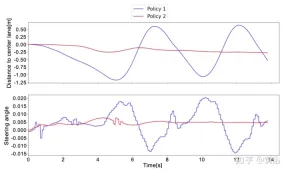
To better understand the difference between Strategy 1 and Strategy 2, here is the steering angle predicted by the neural network and the distance to the center lane within a short window of real-world testing. It can be noticed that the two strategies behave completely different. Strategy 1 (blue curve) is noisy and unsafe compared to strategy 2 (red curve), which proves that the deep response module is important for deployment on truly autonomous vehicles. Strategy is crucial.
To overcome the limitation of RL, which requires millions of segments to reach the optimal solution, pre-training is performed through imitation learning (IL). Furthermore, even though the trend in IL is to train large models, the same small neural network (~1 million parameters) is used, as the idea is to continue training the system using the RL framework to ensure more robustness and generalization capabilities. This way, the usage of hardware resources is not increased, which is crucial considering possible future multi-agent training.
The data set used in the IL training phase is generated by simulated agents that follow a rule-based approach to movement. In particular, for bending, a pure pursuit tracking algorithm is used, where the agent aims to move along a specific waypoint. Instead, use the IDM model to control the longitudinal acceleration of the agent.
To create the dataset, a rule-based agent was moved over four training scenes, saving scalar parameters and four visual inputs every 100 milliseconds. Instead, the output is given by the pure pursuit algorithm and IDM model.
The two horizontal and vertical controls corresponding to the output only represent tuples (μacc, μsa). Therefore, during the IL training phase, the values of the standard deviation (σacc, σsa) are not estimated, nor are the value functions (vacc, vsa) estimated. These features along with the depth response module are learned in the IL RL training phase.
As shown in the figure, it shows the training of the same neural network starting from the pre-training stage (blue curve, IL RL), and compares the results with RL (red curve, pure RL) in four cases. Even though IL RL training requires fewer times than pure RL and the trend is more stable, both methods achieve good success rates (Figure a).
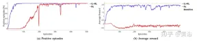
Furthermore, the reward curve shown in Figure b proves that the policy (red curve) obtained using pure RL methods does not even reach an acceptable solution for more training time, while IL RL The policy reaches the optimal solution within a few segments (blue curve in panel b). In this case, the optimal solution is represented by the orange dashed line. This baseline represents the average reward obtained by a simulated agent executing 50,000 segments across 4 scenarios. The simulated agent follows the deterministic rules, which are the same as those used to collect the IL pre-training data set, that is, the pure pursuit rule is used for bending and the IDM rule is used for longitudinal acceleration. The gap between the two approaches may be even more pronounced, training systems to perform more complex maneuvers in which intelligence-body interaction may be required.
The above is the detailed content of Deep reinforcement learning tackles real-world autonomous driving. For more information, please follow other related articles on the PHP Chinese website!

 From Friction To Flow: How AI Is Reshaping Legal WorkMay 09, 2025 am 11:29 AM
The legal tech revolution is gaining momentum, pushing legal professionals to actively embrace AI solutions. Passive resistance is no longer a viable option for those aiming to stay competitive. Why is Technology Adoption Crucial? Legal professional
 This Is What AI Thinks Of You And Knows About YouMay 09, 2025 am 11:24 AM
Many assume interactions with AI are anonymous, a stark contrast to human communication. However, AI actively profiles users during every chat. Every prompt, every word, is analyzed and categorized. Let's explore this critical aspect of the AI revo
 7 Steps To Building A Thriving, AI-Ready Corporate CultureMay 09, 2025 am 11:23 AM
A successful artificial intelligence strategy cannot be separated from strong corporate culture support. As Peter Drucker said, business operations depend on people, and so does the success of artificial intelligence. For organizations that actively embrace artificial intelligence, building a corporate culture that adapts to AI is crucial, and it even determines the success or failure of AI strategies. West Monroe recently released a practical guide to building a thriving AI-friendly corporate culture, and here are some key points: 1. Clarify the success model of AI: First of all, we must have a clear vision of how AI can empower business. An ideal AI operation culture can achieve a natural integration of work processes between humans and AI systems. AI is good at certain tasks, while humans are good at creativity and judgment
 Netflix New Scroll, Meta AI's Game Changers, Neuralink Valued At $8.5 BillionMay 09, 2025 am 11:22 AM
Meta upgrades AI assistant application, and the era of wearable AI is coming! The app, designed to compete with ChatGPT, offers standard AI features such as text, voice interaction, image generation and web search, but has now added geolocation capabilities for the first time. This means that Meta AI knows where you are and what you are viewing when answering your question. It uses your interests, location, profile and activity information to provide the latest situational information that was not possible before. The app also supports real-time translation, which completely changed the AI experience on Ray-Ban glasses and greatly improved its usefulness. The imposition of tariffs on foreign films is a naked exercise of power over the media and culture. If implemented, this will accelerate toward AI and virtual production
 Take These Steps Today To Protect Yourself Against AI CybercrimeMay 09, 2025 am 11:19 AM
Artificial intelligence is revolutionizing the field of cybercrime, which forces us to learn new defensive skills. Cyber criminals are increasingly using powerful artificial intelligence technologies such as deep forgery and intelligent cyberattacks to fraud and destruction at an unprecedented scale. It is reported that 87% of global businesses have been targeted for AI cybercrime over the past year. So, how can we avoid becoming victims of this wave of smart crimes? Let’s explore how to identify risks and take protective measures at the individual and organizational level. How cybercriminals use artificial intelligence As technology advances, criminals are constantly looking for new ways to attack individuals, businesses and governments. The widespread use of artificial intelligence may be the latest aspect, but its potential harm is unprecedented. In particular, artificial intelligence
 A Symbiotic Dance: Navigating Loops Of Artificial And Natural PerceptionMay 09, 2025 am 11:13 AM
The intricate relationship between artificial intelligence (AI) and human intelligence (NI) is best understood as a feedback loop. Humans create AI, training it on data generated by human activity to enhance or replicate human capabilities. This AI
 AI's Biggest Secret — Creators Don't Understand It, Experts SplitMay 09, 2025 am 11:09 AM
Anthropic's recent statement, highlighting the lack of understanding surrounding cutting-edge AI models, has sparked a heated debate among experts. Is this opacity a genuine technological crisis, or simply a temporary hurdle on the path to more soph
 Bulbul-V2 by Sarvam AI: India's Best TTS ModelMay 09, 2025 am 10:52 AM
India is a diverse country with a rich tapestry of languages, making seamless communication across regions a persistent challenge. However, Sarvam’s Bulbul-V2 is helping to bridge this gap with its advanced text-to-speech (TTS) t


Hot AI Tools

Undresser.AI Undress
AI-powered app for creating realistic nude photos

AI Clothes Remover
Online AI tool for removing clothes from photos.

Undress AI Tool
Undress images for free

Clothoff.io
AI clothes remover

Video Face Swap
Swap faces in any video effortlessly with our completely free AI face swap tool!

Hot Article
Hot Tools

SecLists
SecLists is the ultimate security tester's companion. It is a collection of various types of lists that are frequently used during security assessments, all in one place. SecLists helps make security testing more efficient and productive by conveniently providing all the lists a security tester might need. List types include usernames, passwords, URLs, fuzzing payloads, sensitive data patterns, web shells, and more. The tester can simply pull this repository onto a new test machine and he will have access to every type of list he needs.

DVWA
Damn Vulnerable Web App (DVWA) is a PHP/MySQL web application that is very vulnerable. Its main goals are to be an aid for security professionals to test their skills and tools in a legal environment, to help web developers better understand the process of securing web applications, and to help teachers/students teach/learn in a classroom environment Web application security. The goal of DVWA is to practice some of the most common web vulnerabilities through a simple and straightforward interface, with varying degrees of difficulty. Please note that this software

SublimeText3 Mac version
God-level code editing software (SublimeText3)

SublimeText3 English version
Recommended: Win version, supports code prompts!

SublimeText3 Linux new version
SublimeText3 Linux latest version

